Last updated: 2024-11-01

Checks: 7 0

Knit directory: 2021_MPSIIIBvQ96-RNAseq-7dpfLarve/

This reproducible R Markdown analysis was created with workflowr (version 1.7.1). The Checks tab describes the reproducibility checks that were applied when the results were created. The Past versions tab lists the development history.

R Markdown file: up-to-date

Great! Since the R Markdown file has been committed to the Git repository, you know the exact version of the code that produced these results.

Environment: empty

Great job! The global environment was empty. Objects defined in the global environment can affect the analysis in your R Markdown file in unknown ways. For reproduciblity it’s best to always run the code in an empty environment.

Seed: set.seed(20211120)

The command set.seed(20211120) was run prior to running the code in the R Markdown file. Setting a seed ensures that any results that rely on randomness, e.g. subsampling or permutations, are reproducible.

Session information: recorded

Great job! Recording the operating system, R version, and package versions is critical for reproducibility.

Cache: none

Nice! There were no cached chunks for this analysis, so you can be confident that you successfully produced the results during this run.

File paths: relative

Great job! Using relative paths to the files within your workflowr project makes it easier to run your code on other machines.

Repository version: 7bb9ce6

Great! You are using Git for version control. Tracking code development and connecting the code version to the results is critical for reproducibility.

The results in this page were generated with repository version 7bb9ce6. See the Past versions tab to see a history of the changes made to the R Markdown and HTML files.

Note that you need to be careful to ensure that all relevant files for the analysis have been committed to Git prior to generating the results (you can use wflow_publish or wflow_git_commit). workflowr only checks the R Markdown file, but you know if there are other scripts or data files that it depends on. Below is the status of the Git repository when the results were generated:


Ignored files:
    Ignored:    .DS_Store
    Ignored:    .RData
    Ignored:    .Rapp.history
    Ignored:    .Rhistory
    Ignored:    .Rproj.user/
    Ignored:    analysis/.DS_Store
    Ignored:    code/.DS_Store
    Ignored:    code/fromHPC/.DS_Store
    Ignored:    code/fromHPC/smk/.DS_Store
    Ignored:    code/fromHPC/smk/slurm/.DS_Store
    Ignored:    data/.DS_Store
    Ignored:    data/Nhi_data/.DS_Store
    Ignored:    data/R_objects/.DS_Store
    Ignored:    data/R_objects/larvae/.DS_Store
    Ignored:    data/adult_brain/.DS_Store
    Ignored:    data/adult_brain/05_featureCounts/.DS_Store
    Ignored:    data/adult_brain/fastqc_raw/.DS_Store
    Ignored:    data/gene_sets/.DS_Store
    Ignored:    data/larvae/.DS_Store
    Ignored:    data/larvae/fastqc_align/.DS_Store
    Ignored:    data/larvae/fastqc_align_dedup/.DS_Store
    Ignored:    data/larvae/fastqc_raw/.DS_Store
    Ignored:    data/larvae/fastqc_trim/.DS_Store
    Ignored:    data/larvae/featureCounts/.DS_Store
    Ignored:    data/larvae/meta/.DS_Store
    Ignored:    data/larvae/starAlignLog/.DS_Store
    Ignored:    output/.DS_Store
    Ignored:    output/plots/
    Ignored:    output/plots4poster/.DS_Store
    Ignored:    output/plots4pub/

Untracked files:
    Untracked:  Rplot01.pdf
    Untracked:  Rplot02.png
    Untracked:  code/6mBrain_RNAseq_genoSex.rmd
    Untracked:  code/6mBrain_fems.rmd
    Untracked:  code/HS.R
    Untracked:  code/about.Rmd
    Untracked:  code/analysis.Rmd
    Untracked:  code/analysis_final.rmd
    Untracked:  code/analysis_final_v2.rmd
    Untracked:  code/checkGenotypes.rmd
    Untracked:  code/explorationRUV.Rmd
    Untracked:  code/genotypeCheck.Rmd
    Untracked:  code/license.Rmd
    Untracked:  code/nhi6mdata.rmd
    Untracked:  code/plots4pub2.rmd
    Untracked:  code/plots4pub_RNAseq_afterreview1.R
    Untracked:  code/wgcna.rmd
    Untracked:  data/R_objects/adult_brain/HMPKEGG_6m_brain_genosex_CQN.rds
    Untracked:  data/R_objects/adult_brain/HMP_ire_6m_brain_genosex_CQN.rds
    Untracked:  data/R_objects/adult_brain/cqn_logCPM_6m_brain.rds
    Untracked:  data/R_objects/adult_brain/dge_6m_brain_cqn.rds
    Untracked:  data/R_objects/adult_brain/fry_cell_6m_brain_genosex_CQN.rds
    Untracked:  data/R_objects/adult_brain/fry_cell_RNAseq.rds
    Untracked:  data/R_objects/adult_brain/goseqtibbles_6m_brain_genosex_CQN.rds
    Untracked:  data/R_objects/adult_brain/hmp.kegg.rna.rds
    Untracked:  data/R_objects/adult_brain/toptablescqn_bysex.rds
    Untracked:  data/allLLIDs.rds
    Untracked:  data/ensembl_zebrafish.rds
    Untracked:  data/proteomics/
    Untracked:  data/with_go_evidence.rds
    Untracked:  dre00020.pathview.multi.png
    Untracked:  dre00020.png
    Untracked:  dre00020.xml
    Untracked:  hsa04650.EOfADproteomes.multi.png
    Untracked:  hsa04650.MPSIIIBproteomes.multi.png
    Untracked:  hsa04650.png
    Untracked:  hsa04650.xml
    Untracked:  hsa04666.EOfADproteomes.multi.png
    Untracked:  hsa04666.MPSIIIBproteomes.multi.png
    Untracked:  hsa04666.png
    Untracked:  hsa04666.xml
    Untracked:  larvae dre00020.pathview.multi.png
    Untracked:  output/DE_proteins_for_string/
    Untracked:  output/GOenrichment_enrichmentTable.csv
    Untracked:  output/plots4RADposter/
    Untracked:  output/plots4kim/
    Untracked:  output/plots4pub2/
    Untracked:  output/plots4pub3/
    Untracked:  output/spreadsheets/RNAseqlarvae_celltypeFry.xlsx
    Untracked:  output/spreadsheets/RNAseqlarvae_hmpoutputs.xlsx
    Untracked:  output/spreadsheets/geneset_RNAseq_v2.xlsx
    Untracked:  output/spreadsheets/goseq_RNAseq_v2.xlsx
    Untracked:  output/spreadsheets/limma_proteomics_6mbrain.xlsx
    Untracked:  output/spreadsheets/proteomics_6mbrain_hmpoutputs.xlsx
    Untracked:  output/spreadsheets/toptables_RNAseq_v2.xlsx
    Untracked:  temp.png

Unstaged changes:
    Deleted:    analysis/6mBrain_fems.rmd
    Deleted:    analysis/HS.R
    Deleted:    analysis/about.Rmd
    Deleted:    analysis/analysis.Rmd
    Deleted:    analysis/analysis_adultbrain.knit.md
    Deleted:    analysis/analysis_final.rmd
    Deleted:    analysis/checkGenotypes.rmd
    Deleted:    analysis/explorationRUV.Rmd
    Deleted:    analysis/genotypeCheck.Rmd
    Deleted:    analysis/license.Rmd
    Deleted:    analysis/nhi6mdata.rmd
    Deleted:    analysis/plots4pub2.rmd
    Modified:   data/R_objects/adult_brain/dge.rds
    Modified:   data/R_objects/adult_brain/hmp_ire.rds
    Modified:   data/R_objects/adult_brain/logcpm.rds
    Modified:   data/R_objects/larvae/celltype_larvae.rds
    Modified:   data/R_objects/larvae/dge.rds
    Modified:   data/R_objects/larvae/hmp_ire.rds
    Modified:   data/R_objects/larvae/hmp_kegg.rds
    Modified:   data/R_objects/larvae/logcpm.rds
    Modified:   data/R_objects/larvae/toptablescqn.rds
    Modified:   data/adult_brain/karissas_metadata.xlsx
    Modified:   output/spreadsheets/toptables_cqn.xlsx

Note that any generated files, e.g. HTML, png, CSS, etc., are not included in this status report because it is ok for generated content to have uncommitted changes.

These are the previous versions of the repository in which changes were made to the R Markdown (analysis/analysis_adultbrain.rmd) and HTML (docs/analysis_adultbrain.html) files. If you’ve configured a remote Git repository (see ?wflow_git_remote), click on the hyperlinks in the table below to view the files as they were in that past version.

File	Version	Author	Date	Message
Rmd	7bb9ce6	Karissa Barthelson	2024-11-01	wflow_publish("analysis/*")
Rmd	6e89e87	Karissa Barthelson	2023-09-02	final analysis complete
Rmd	9f57eae	Karissa Barthelson	2023-04-28	test
Rmd	973da7b	Karissa Barthelson	2023-03-09	Message that describes what this change does
Rmd	6d8b85a	Karissa Barthelson	2023-03-03	added adult brain

library(tidyverse)
library(magrittr)
library(readxl)
library(ngsReports)
library(AnnotationHub)
library(pander)
library(scales)
library(pheatmap)
library(ggpubr)
library(msigdbr)
library(scales)
library(ggrepel)
library(ggfortify)
library(RColorBrewer)
library(ComplexHeatmap)
library(tidyHeatmap)
library(circlize)
library(UpSetR)
library(edgeR)
library(goseq)
library(fgsea)
library(cqn)
library(kableExtra)
library(harmonicmeanp)
library(ssizeRNA)

theme_set(
  theme_bw() +
    theme(
      plot.title = element_text(hjust = 0.5)
    ))

Read in data

ah <- AnnotationHub() %>%
    subset(species == "Danio rerio") %>%
    subset(rdataclass == "EnsDb")

ensDb <- ah[["AH83189"]] # for release 101, latest version and the alignment
grTrans <- transcripts(ensDb)
trLengths <- exonsBy(ensDb, "tx") %>%
    width() %>%
    vapply(sum, integer(1))
mcols(grTrans)$length <- trLengths[names(grTrans)]
gcGene <- grTrans %>%
  mcols() %>%
  as.data.frame() %>%
  dplyr::select(gene_id, tx_id, gc_content, length) %>%
  as_tibble() %>%
  group_by(gene_id) %>%
  summarise(
    gc_content = sum(gc_content*length) / sum(length),
    length = ceiling(median(length))
  )
grGenes <- genes(ensDb)
mcols(grGenes) %<>%
  as.data.frame() %>%
  left_join(gcGene) %>%
  as.data.frame() %>%
  DataFrame()

# readin meta and tidy up columns
meta <- read_excel("data/adult_brain/karissas_metadata.xlsx", sheet = "onlyseq") %>% 
  mutate(genotype = case_when(
    `usable genotype?` == "wt" ~ "wt", 
    `usable genotype?` == "EOfAD" ~ "EOfADlike", 
    `usable genotype?` == "MPS-III" ~ "MPSIIIB"
  ) %>% 
    factor(levels = c("wt",  "EOfADlike", "MPSIIIB")), 
  tank = as.factor(tank), 
  sex  = as.factor(sex),
  sample = paste0(fish, "_", genotype), 
  group = paste0(genotype, "_", sex) %>% as.factor(),
  age = "6 m adult brain",
  RIN = as.numeric(`RIN/DIN`)
  ) %>% 
  dplyr::select(
    # reorder the metadata nicely
    fish,genotype,sex,group,batch,tank,RIN,everything()
    ) %>% 
  as_tibble()

# read in counts and cleanup
featureCounts <- 
  read_delim("data/adult_brain/05_featureCounts/counts.out", delim = "\t", skip = 1) %>%
  set_names(basename(names(.))) %>% 
  set_names(names(.) %>% str_remove(pattern = "_S[0-9]+_merged.Aligned.sortedByCoord.dedup.out.bam")) %>% 
  as_tibble() %>% 
  dplyr::select(-c(Chr, Start, End, Length, Strand)) %>% 
  gather(key = "ULN", value = "counts", starts_with("22")) %>% 
  left_join(meta) %>% 
  mutate(sample = paste0(fish, "_", genotype)) %>% 
  dplyr::select(Geneid, counts, sample) %>% 
  spread(key = "sample", value = "counts") %>% 
  column_to_rownames("Geneid") %>% 
  .[,1:24]

filter lowly expressed genes

Genes which are lowly expressed are considered uninformative for de analysis. Here, we set the threshold to be a min CPM of 0.5 (following the 10/min lib size rule proposed by gordon smyth). The effect of filtering is found below.

DGEList objects were created, which brings together the sample metadata and counts in each experiment. TMM normalisation to the counts is also applied when making these objects.

a <- featureCounts %>% 
    cpm(log = TRUE) %>%
    as.data.frame() %>% 
  pivot_longer(
    cols = everything(),
    names_to = "sample",
    values_to = "logCPM"
  ) %>%
  split(f = .$sample) %>%
  lapply(function(x){
    d <- density(x$logCPM)
    tibble(
      sample = unique(x$sample),
      x = d$x,
      y = d$y
    )
  }) %>%
  bind_rows() %>%
  left_join(meta) %>% 
  ggplot(aes(x, y, colour = genotype, group = sample)) +
  geom_line() +
  labs(
    x = "logCPM",
    y = "Density",
    colour = "genotype"
  )+
  ggtitle("Before filtering") +
  theme_bw()
b <- featureCounts %>% 
  .[rowSums(cpm(.) >= 0.5) >= 8,] %>% 
    cpm(log = TRUE) %>%
    as.data.frame() %>% 
  pivot_longer(
    cols = everything(),
    names_to = "sample",
    values_to = "logCPM"
  ) %>%
  split(f = .$sample) %>%
  lapply(function(x){
    d <- density(x$logCPM)
    tibble(
      sample = unique(x$sample),
      x = d$x,
      y = d$y
    )
  }) %>%
  bind_rows() %>%
  left_join(meta) %>% 
  ggplot(aes(x, y, colour = genotype, group = sample)) +
  geom_line() +
  labs(
    x = "logCPM",
    y = "Density",
    colour = "genotype"
  )+
  ggtitle("After filtering")

ggarrange(a, b, common.legend = TRUE)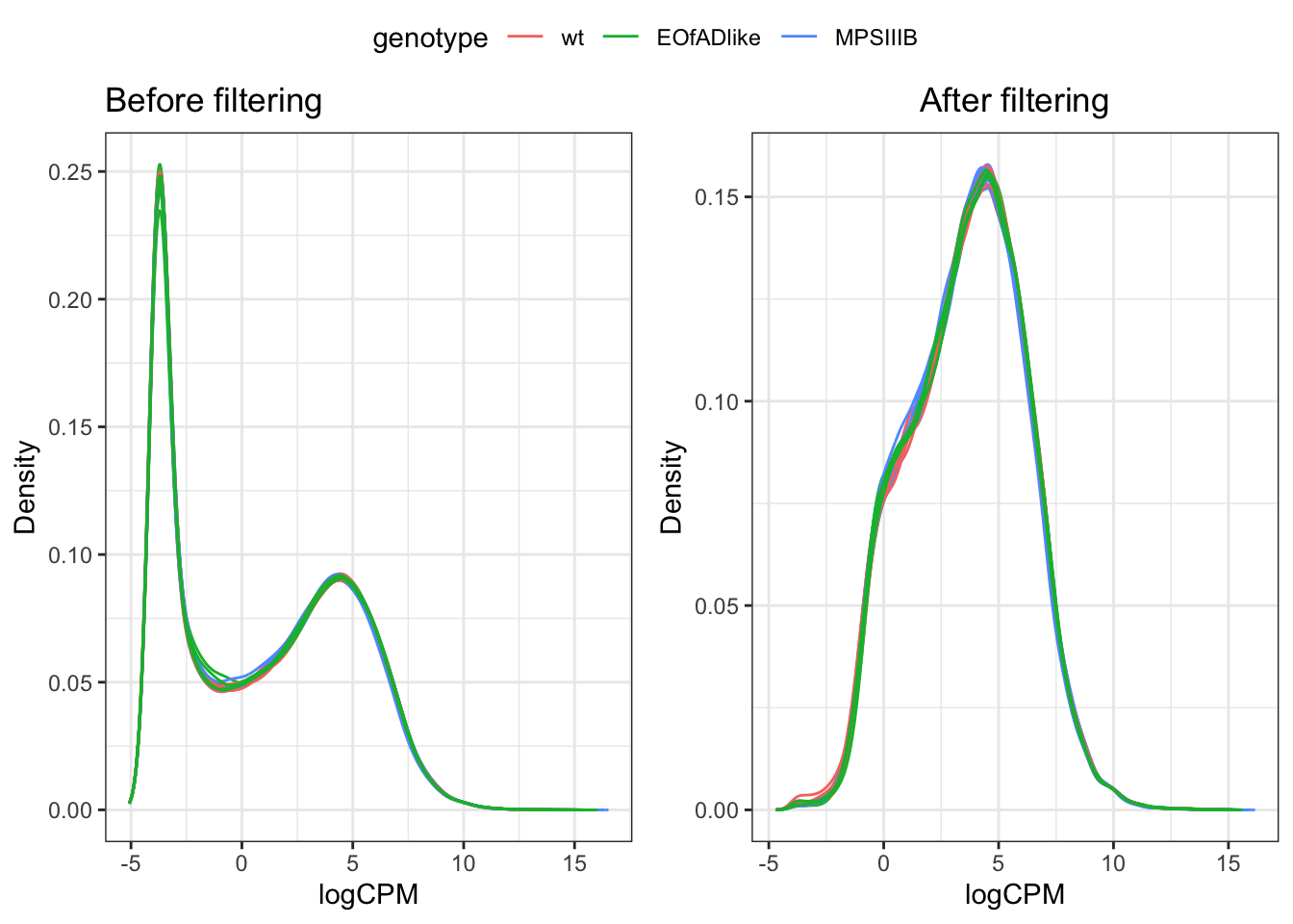

x <- featureCounts %>% 
  as.matrix() %>% 
 .[rowSums(cpm(.) >= 0.5) >= 8,] %>%
  DGEList(
    samples = tibble(sample = colnames(.)) %>%
      left_join(meta),
    genes = grGenes[rownames(.)] %>%
      as.data.frame() %>%
      dplyr::select(
        chromosome = seqnames, start, end, 
        gene_id, gene_name, gene_biotype, description, entrezid
      ) %>% 
      left_join(gcGene) %>% 
      as_tibble()
  ) %>%
  calcNormFactors()

PCA

I first want to explore the overall similarity between samples by PCA. No distinct clusters of samples are observed. However, there might be some subtle seperatation of the MPS IIIB mutants.

x %>% 
  cpm(log=TRUE) %>% 
  t() %>% 
  prcomp() %>% 
  autoplot(data = tibble(sample = rownames(.$x)) %>%
      left_join(x$samples),
    colour = "genotype", 
    shape = "sex",
    size = 6
  ) +
  theme(aspect.ratio = 1) +
  labs(colour = "genotype")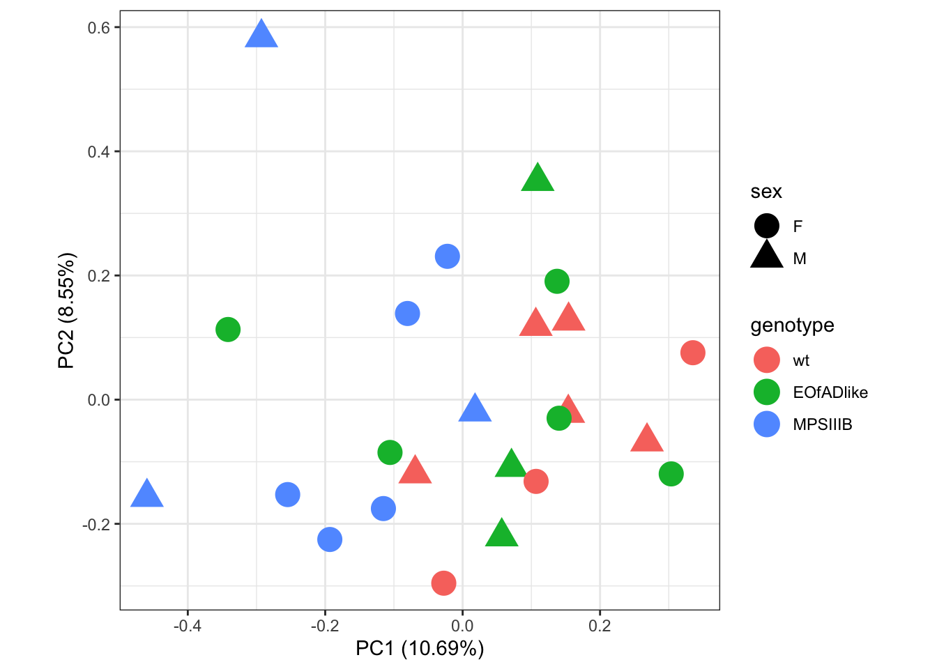

x$counts %>% 
  cpm(log=TRUE) %>% 
  t() %>% 
  prcomp() %>% 
  autoplot(data = tibble(sample = rownames(.$x)) %>%
      left_join(x$samples),
    colour = "sex", 
    size = 6
  ) +
  theme(aspect.ratio = 1) +
  labs(colour = "Sex")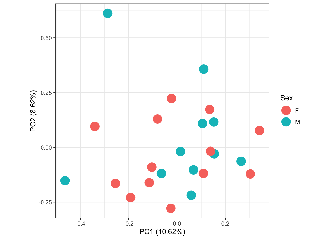

x$counts %>% 
  cpm(log=TRUE) %>% 
  t() %>% 
  prcomp() %>% 
  autoplot(data = tibble(sample = rownames(.$x)) %>%
      left_join(x$samples),
    colour = "tank", 
    size = 6
  ) +
  theme(aspect.ratio = 1) +
  labs(colour = "Tank")

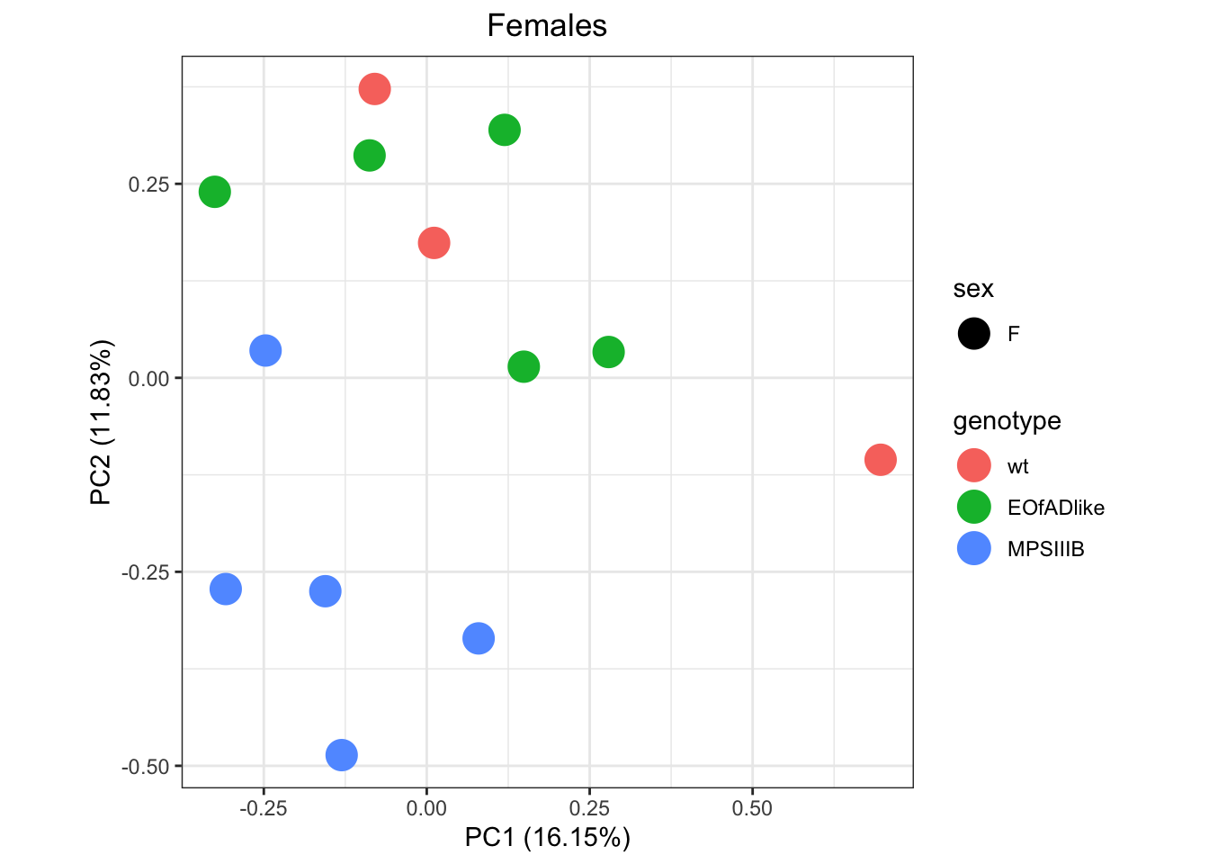
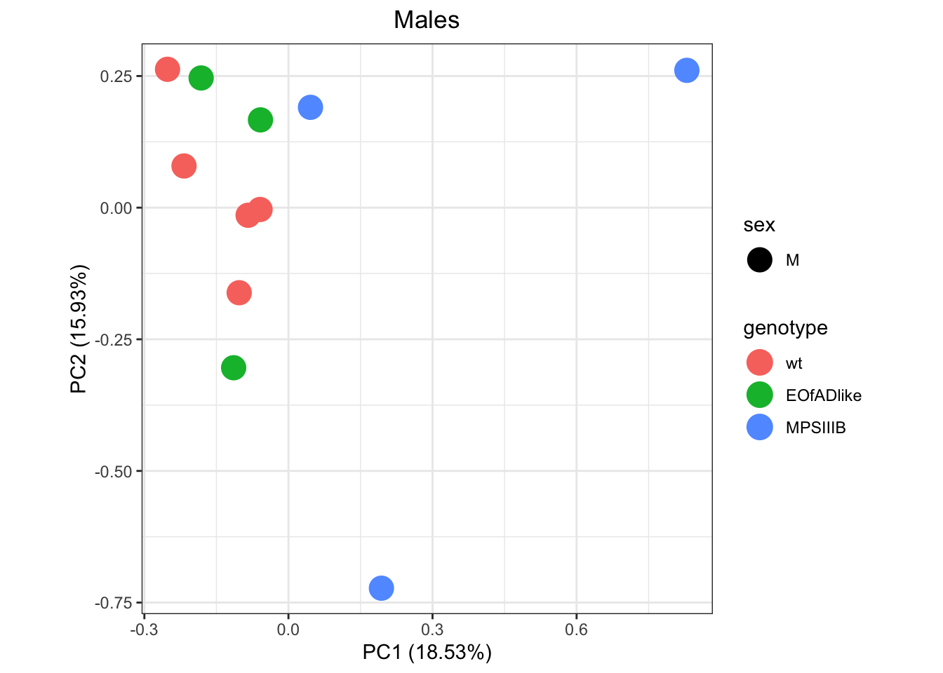
within sexes

Since it is a bit hard to see whats going on within sexes, I will next perform PCAs on each sex seperately

fem.samples <- x$samples %>% 
  dplyr::filter(sex == "F") %>% 
  rownames()

male.samples <- x$samples %>% 
  dplyr::filter(sex == "M") %>% 
  rownames()

x %>% 
  cpm(log = TRUE) %>% 
  .[,fem.samples] %>% 
  t %>% 
  prcomp() %>% 
  autoplot(data = tibble(sample = rownames(.$x)) %>%
             left_join(x$samples),
           colour = "genotype",
           shape = "sex", 
           size = 6
  ) +
  theme(aspect.ratio = 1) +
  labs(
    title = "Females"
  )

x %>% 
  cpm(log = TRUE) %>% 
  .[,male.samples] %>% 
  t %>% 
  prcomp() %>% 
  autoplot(data = tibble(sample = rownames(.$x)) %>%
             left_join(x$samples),
           colour = "genotype",
           shape = "sex", 
           size = 6
  ) +
  theme(aspect.ratio = 1) +
  labs(
    title = "Males"
  )

Initial DE analysis to check for %GC and length bias

For this analysis, I will keep the model matrix simple and look at only effect of genotype. This should be sufficient to look for bias due to GC and length, ans so whether CQN is required.

design.simple <- model.matrix(~genotype, data = x$samples) %>% 
  set_colnames(gsub(colnames(.), pattern = "genotype", replacement = ""))

fit_1 <- x %>% 
  estimateDisp(design.simple) %>% 
  glmFit(design.simple)

toptable_1 <- design.simple %>% colnames() %>% .[2:3] %>%
  sapply(function(x){
    glmLRT(fit_1, coef = x) %>%
      topTags(n = Inf) %>%
      .[["table"]] %>%
      as_tibble() %>%
      arrange(PValue) %>%
       mutate(
        coef = x,
        DE = FDR < 0.05
      ) %>% 
      dplyr::select(
        gene_name, logFC, logCPM, PValue, FDR, DE, everything()  
      )
      
  }, simplify = FALSE)

toptable_1 %>%
  bind_rows() %>% 
  ggplot(aes(y = -log10(PValue), x = logFC, colour = DE)) +
  geom_point(
    alpha = 0.5, size = 1.25
  ) +
  facet_wrap(~coef) +
  # geom_label_repel(
  #   aes(label = gene_name),
  #   data = .  %>% dplyr::filter(FDR < 0.05),
  #   show.legend = FALSE
  #   ) +
  coord_cartesian(xlim = c(-2.5,2.5), 
                  ylim = c(0, 20) )+
  theme(legend.position = "none") +
  scale_color_manual(values = c("grey50", "red"))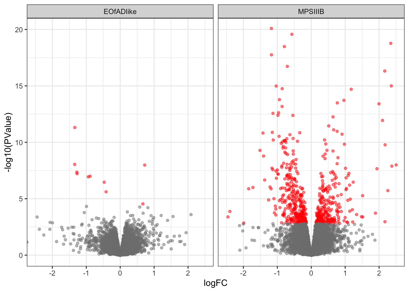

toptable_1 %>%
  bind_rows() %>% 
  ggplot(aes(x = logCPM, y = logFC,  colour = DE)) +
  geom_point(
    alpha = 0.5
  ) +
  
  facet_wrap(~coef) +
  # geom_label_repel(
  #   aes(label = gene_name), 
  #   data = .  %>% dplyr::filter(FDR < 0.05), 
  #   show.legend = FALSE
  #   ) +
  theme(legend.position = "none") +
  scale_color_manual(values = c("grey50", "red"))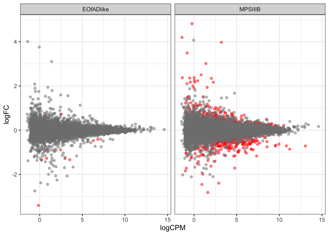

Vis

ggarrange(
toptable_1 %>% 
  bind_rows() %>% 
  mutate(rankstat = sign(logFC)*-log10(PValue)) %>% 
  ggplot(aes(x = length, y = rankstat)) +
  geom_point(
    aes(colour = DE),
    alpha = 0.5
  ) +
  geom_smooth(se = FALSE, method = "gam") +
  facet_grid(rows = vars(coef)) +
  theme_bw() +
  theme(legend.position = "none") +
  scale_color_manual(values = c("grey50", "red")) +
  scale_x_log10()+
  labs(x = "Average transcript length per gene",
       colour = "Differentially expressed?",
       y = "sign(logFC)*-log10(PValue)") +
  coord_cartesian(ylim = c(-10, 10)),

toptable_1 %>% 
  bind_rows() %>% 
  mutate(rankstat = sign(logFC)*-log10(PValue)) %>% 
  ggplot(aes(x = gc_content, y = rankstat)) +
  geom_point(
    aes(colour = DE),
    alpha = 0.5
  ) +
  geom_smooth(se = FALSE, method = "gam") +
  facet_grid(rows = vars(coef)) +
  theme_bw() +
  theme(legend.position = "none") +
  scale_color_manual(values = c("grey50", "red")) +
  coord_cartesian(ylim = c(-10,10)) + 
  labs(x = "Weighted average GC content (%) per gene", 
       colour = "Differentially expressed?", 
       y = "sign(logFC)*-log10(PValue)"),
common.legend = TRUE, 
labels = "AUTO"
)

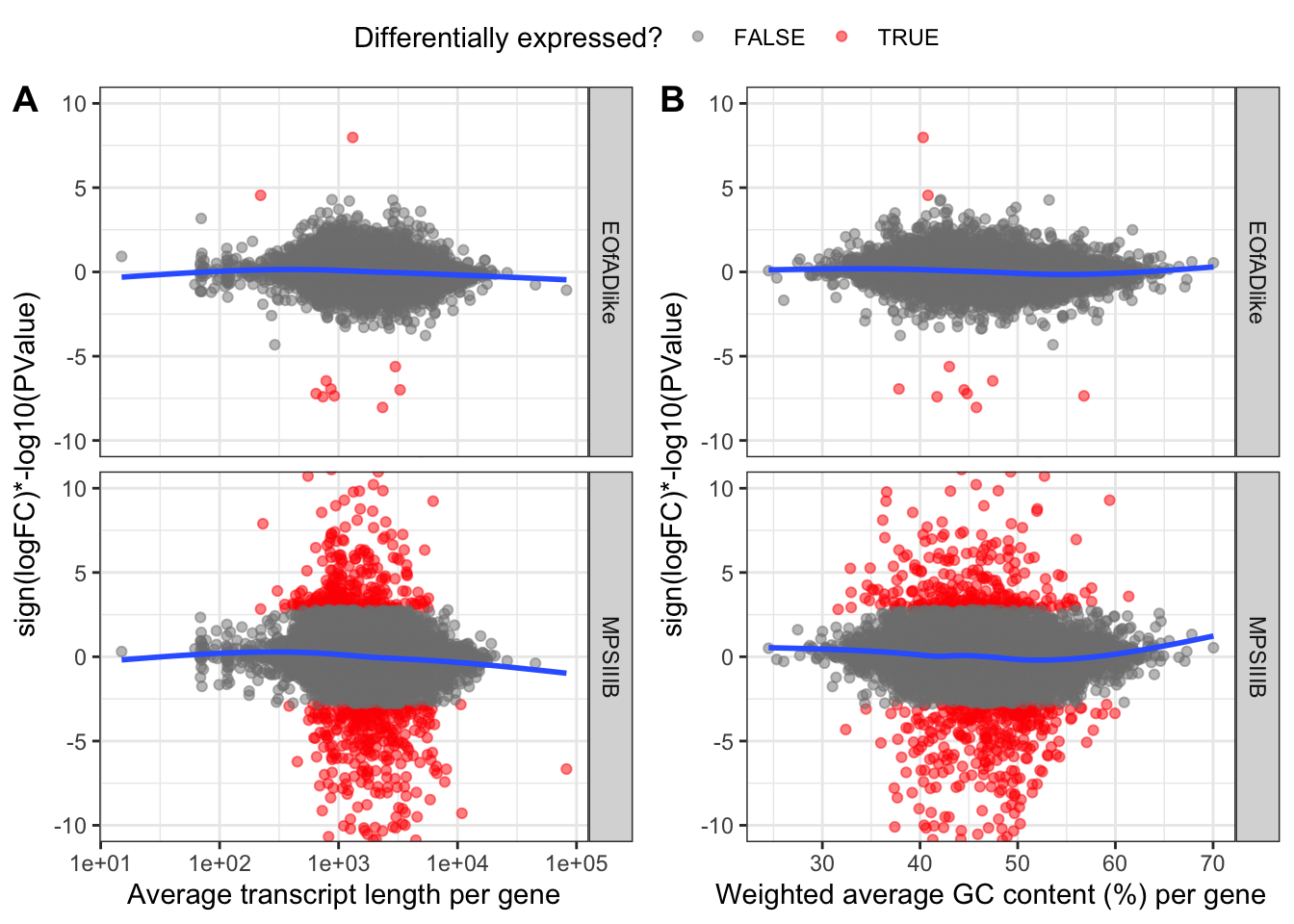
CQN

Some bias is observed, and so CQN will be applied.

cqn <- 
  x %>% 
  with(
    cqn(
      counts = counts,
      x = genes$gc_content,
      lengths = genes$length,
      sizeFactors = samples$lib.size
    )
  )
# 
logCPM <- cqn$y + cqn$offset

plot out the model fits

par(mfrow = c(1, 2))
cqnplot(cqn, n = 1, xlab = "GC Content")
cqnplot(cqn, n = 2, xlab = "Length")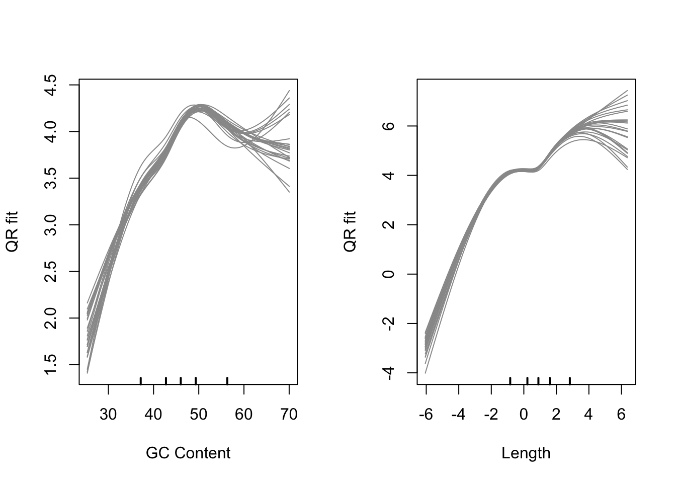

Model fits for GC content and gene length under the CQN model. Variability is clearly visible at either end

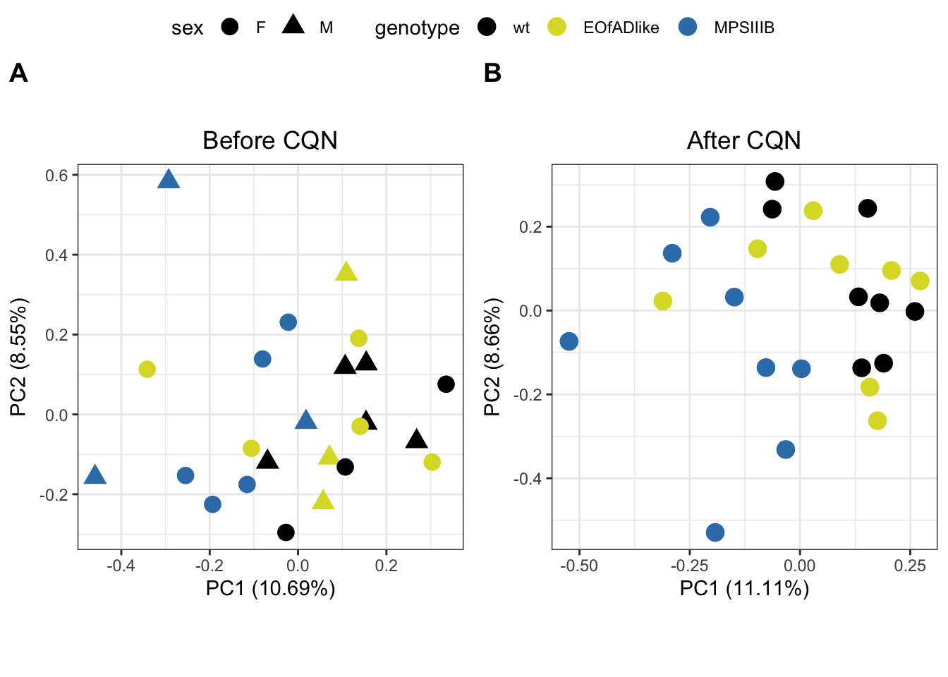
par(mfrow = c(1, 1))

PCA after cqn

PCA analysis was repeated. Similar clustering of samples was observed, with MPS-IIIA samples appearing to form a more distinct cluster from the rest of the samples. The sgsh/+ samples appear much more variable.

genocols = c("#000000", "#DBDB2F", "#377EB8")

ggarrange(
  cpm(x, log = T) %>%
    t() %>%
    prcomp() %>% 
    autoplot(data = tibble(sample = rownames(.$x)) %>%
               left_join(x$samples),
             colour = "genotype", 
             shape = "sex", 
             size = 4
    ) +
    scale_colour_manual(values = genocols) +
    theme(aspect.ratio = 1) +
    ggtitle("Before CQN"),
  
  logCPM %>% 
    t() %>% 
    prcomp() %>%
    autoplot(data = tibble(sample = rownames(.$x)) %>%
               left_join(x$samples),
             colour = "genotype", 
             size = 4
    ) +
    scale_colour_manual(values = genocols) +
    theme(aspect.ratio = 1) +
    ggtitle("After CQN"),
  common.legend = T, 
  labels = "AUTO"
)

#ggsave("plotsforpub/PCA_cqn.png", width = 18, height = 8, units = "cm", scale = 1.4)

DE with cqn

The DE analysis was then repeated, this time including the offset generated by cqn in the model.

Will also create a new design and contrasts matrices to be able to determine the DEGs within sexes.

# Add the offset to the dge object 
x$offset <- cqn$glm.offset

# new desing matrix
design.bygroup <- 
  model.matrix(~0 + group, data = x$samples %>% 
                 droplevels()) %>% 
   set_colnames(gsub(colnames(.), pattern = "group", replacement = ""))


contrasts <- makeContrasts( 
 
  MPSIIIB_M - wt_M , # effect of MPS IIIB in males
  MPSIIIB_F - wt_F, # effect of MPS IIIB in females
  
  EOfADlike_M - wt_M, # effect of EOfAD in males
  EOfADlike_F - wt_F, # effect of EOfAD in females

  levels = design.bygroup
  )

# fit the glm
fit_cqn_simple <- x %>% 
  estimateDisp(design.simple) %>% 
  glmFit(design.simple)

fit_cqn_bysex <- x %>% 
  estimateDisp(design.bygroup) %>% 
  glmFit(design.bygroup)

# call toptables 
toptables_cqn_simple <- design.simple %>% colnames() %>% .[2:3] %>% 
  sapply(function(x){
    glmLRT(fit_cqn_simple, coef = x) %>%
      topTags(n = Inf) %>%
      .[["table"]] %>%
      as_tibble() %>%
      arrange(PValue) %>%
       mutate(
        coef = x,
        DE = FDR < 0.05
      ) %>% 
      dplyr::select(
        gene_name, logFC, logCPM, PValue, FDR, DE, everything()  
      )
      
  }, simplify = FALSE)

toptables_cqn_bygroup <- 
  colnames(contrasts) %>% 
  sapply(function(x) {
    glmLRT(fit_cqn_bysex, contrast = contrasts[,x]) %>% 
      topTags(n = Inf)  %>% 
      .[["table"]] %>%
      as_tibble() %>%
      arrange(PValue) %>%
      mutate(
        coef = x,
        coef = str_remove(coef, pattern = " - .+"),
        DE = FDR < 0.05
      ) %>% 
      dplyr::select(
        gene_name, logFC, logCPM, PValue, FDR, DE, everything()
      )
        }, simplify = FALSE)

# tidy up the names of this. 
names(toptables_cqn_bygroup) %<>% 
  str_remove(pattern = " - .+")

Visualisation

tables of n DE

toptables_cqn_bygroup %>% 
  lapply(function(y) {
    y %>% 
      mutate(
      direction = sign(logFC), .after = logFC
      ) %>% 
      dplyr::filter(DE == TRUE) %>% 
      group_by(direction) %>% 
      summarise(n = n())
  })

$MPSIIIB_M
# A tibble: 2 × 2
  direction     n
      <dbl> <int>
1        -1   141
2         1   212

$MPSIIIB_F
# A tibble: 2 × 2
  direction     n
      <dbl> <int>
1        -1   123
2         1    77

$EOfADlike_M
# A tibble: 2 × 2
  direction     n
      <dbl> <int>
1        -1     3
2         1     1

$EOfADlike_F
# A tibble: 2 × 2
  direction     n
      <dbl> <int>
1        -1    11
2         1     1

toptables_cqn_bygroup %>% lapply(dplyr::filter, DE == T)

$MPSIIIB_M
# A tibble: 353 × 17
   gene_name      logFC  logCPM   PValue      FDR DE    chromosome  start    end
   <chr>          <dbl>   <dbl>    <dbl>    <dbl> <lgl> <fct>       <int>  <int>
 1 tmem14cb      -3.10   1.62   1.12e-31 2.14e-27 TRUE  24         3.61e7 3.61e7
 2 si:ch1073-16…  4.26  -0.244  2.77e-27 2.64e-23 TRUE  24         3.86e7 3.87e7
 3 im:7160594     1.00   3.14   1.47e-22 9.32e-19 TRUE  24         3.92e7 3.92e7
 4 dnaaf3l        2.04   0.439  4.81e-22 2.29e-18 TRUE  24         3.69e7 3.69e7
 5 mybpc2b        5.39   3.21   3.10e-17 1.18e-13 TRUE  24         3.83e7 3.83e7
 6 CU651662.1     2.62   2.03   1.43e-16 4.55e-13 TRUE  7          7.15e7 7.15e7
 7 tspan36        1.21   2.78   1.37e-13 3.73e-10 TRUE  8          2.97e7 2.97e7
 8 si:ch211-234… -0.826  4.14   3.55e-13 8.45e-10 TRUE  24         3.82e7 3.82e7
 9 cluap1        -0.613  4.54   4.46e-13 9.23e-10 TRUE  24         3.75e7 3.75e7
10 sb:cb1058      2.01   0.0176 4.84e-13 9.23e-10 TRUE  7          2.50e7 2.50e7
# ℹ 343 more rows
# ℹ 8 more variables: gene_id <chr>, gene_biotype <chr>, description <chr>,
#   entrezid <named list>, gc_content <dbl>, length <dbl>, LR <dbl>, coef <chr>

$MPSIIIB_F
# A tibble: 200 × 17
   gene_name      logFC  logCPM   PValue      FDR DE    chromosome  start    end
   <chr>          <dbl>   <dbl>    <dbl>    <dbl> <lgl> <fct>       <int>  <int>
 1 tmem14cb      -2.86   1.62   6.55e-38 1.25e-33 TRUE  24         3.61e7 3.61e7
 2 dnaaf3l        2.07   0.439  2.92e-19 2.78e-15 TRUE  24         3.69e7 3.69e7
 3 si:ch1073-16…  3.08  -0.244  9.15e-19 5.82e-15 TRUE  24         3.86e7 3.87e7
 4 cluap1        -0.619  4.54   4.56e-14 2.17e-10 TRUE  24         3.75e7 3.75e7
 5 mybphb        -1.72   1.98   6.77e-14 2.58e-10 TRUE  6          5.50e7 5.51e7
 6 c7b           -1.60   4.77   8.06e-13 2.56e- 9 TRUE  21         2.09e7 2.09e7
 7 plp1a         -1.20   4.65   1.37e-12 3.74e- 9 TRUE  14         1.46e7 1.46e7
 8 sb:cb1058      2.20   0.0176 7.54e-12 1.80e- 8 TRUE  7          2.50e7 2.50e7
 9 bri3           0.672  5.53   1.32e-11 2.79e- 8 TRUE  3          6.14e7 6.14e7
10 gpd1c          1.43   1.56   1.75e-11 3.33e- 8 TRUE  19         3.18e5 3.26e5
# ℹ 190 more rows
# ℹ 8 more variables: gene_id <chr>, gene_biotype <chr>, description <chr>,
#   entrezid <named list>, gc_content <dbl>, length <dbl>, LR <dbl>, coef <chr>

$EOfADlike_M
# A tibble: 4 × 17
  gene_name         logFC logCPM   PValue     FDR DE    chromosome  start    end
  <chr>             <dbl>  <dbl>    <dbl>   <dbl> <lgl> <fct>       <int>  <int>
1 nenf              0.958  2.53  3.12e-10 5.94e-6 TRUE  17         4.54e7 4.54e7
2 zgc:172014       -3.18  -0.146 1.05e- 6 1.00e-2 TRUE  4          3.08e7 3.08e7
3 col12a1a         -1.43   3.53  4.52e- 6 2.87e-2 TRUE  17         4.98e7 5.00e7
4 si:dkey-170l10.1 -1.13   0.832 1.03e- 5 4.93e-2 TRUE  17         3.16e7 3.16e7
# ℹ 8 more variables: gene_id <chr>, gene_biotype <chr>, description <chr>,
#   entrezid <named list>, gc_content <dbl>, length <dbl>, LR <dbl>, coef <chr>

$EOfADlike_F
# A tibble: 12 × 17
   gene_name        logFC  logCPM  PValue     FDR DE    chromosome  start    end
   <chr>            <dbl>   <dbl>   <dbl>   <dbl> <lgl> <fct>       <int>  <int>
 1 si:dkey-13p1.3   -1.61  0.215  1.76e-9 3.36e-5 TRUE  17         3.16e7 3.16e7
 2 si:ch211-213a13… -3.47  1.87   9.97e-9 9.51e-5 TRUE  22         8.98e6 9.00e6
 3 si:dkey-71b5.7   -3.46  0.926  4.05e-7 2.57e-3 TRUE  16         2.19e7 2.20e7
 4 si:ch211-213a13… -2.91  1.14   9.49e-7 3.98e-3 TRUE  22         9.06e6 9.10e6
 5 traf3ip2l        -3.19  1.04   1.04e-6 3.98e-3 TRUE  6          3.69e7 3.69e7
 6 si:dkey-253d23.4 -2.51  1.70   1.25e-6 3.98e-3 TRUE  22         9.87e6 9.88e6
 7 mybpc2b          -2.84  3.21   2.19e-6 5.96e-3 TRUE  24         3.83e7 3.83e7
 8 si:ch211-261n11… -2.68  1.41   4.11e-6 9.79e-3 TRUE  8          2.25e7 2.25e7
 9 BX322618.1       -2.71  2.91   2.13e-5 4.24e-2 TRUE  20         1.22e7 1.22e7
10 si:ch73-21k16.5   1.12  3.88   2.39e-5 4.24e-2 TRUE  20         4.69e7 4.69e7
11 rad51            -1.61  2.13   2.45e-5 4.24e-2 TRUE  20         4.64e7 4.64e7
12 timm23b          -1.94 -0.0258 2.67e-5 4.24e-2 TRUE  13         3.88e6 3.93e6
# ℹ 8 more variables: gene_id <chr>, gene_biotype <chr>, description <chr>,
#   entrezid <named list>, gc_content <dbl>, length <dbl>, LR <dbl>, coef <chr>

toptables_cqn_simple %>% 
  lapply(function(y) {
    y %>% 
      mutate(
      direction = sign(logFC), .after = logFC
      ) %>% 
      dplyr::filter(DE == TRUE) %>% 
      group_by(direction) %>% 
      summarise(n = n())
  })

$EOfADlike
# A tibble: 2 × 2
  direction     n
      <dbl> <int>
1        -1    10
2         1     1

$MPSIIIB
# A tibble: 2 × 2
  direction     n
      <dbl> <int>
1        -1   333
2         1   284

Volcano plot

toptables_cqn_simple %>%
  bind_rows() %>% 
  ggplot(aes(y = -log10(PValue), x = logFC, colour = DE)) +
  geom_point(
    alpha = 0.5, size = 1.25
  ) +
  facet_wrap(~coef) +
  # geom_label_repel(
  #   aes(label = gene_name),
  #   data = .  %>% dplyr::filter(FDR < 0.05),
  #   show.legend = FALSE
  #   ) +
  coord_cartesian(xlim = c(-2.5,2.5), 
                  ylim = c(0, 20) )+
  theme(legend.position = "none") +
  scale_color_manual(values = c("grey50", "red"))

toptables_cqn_bygroup %>%
  bind_rows() %>% 
  ggplot(aes(y = -log10(PValue), x = logFC, colour = DE)) +
  geom_point(
    alpha = 0.5, size = 1.25
  ) +
  facet_wrap(~coef) +
  # geom_label_repel(
  #   aes(label = gene_name),
  #   data = .  %>% dplyr::filter(FDR < 0.05),
  #   show.legend = FALSE
  #   ) +
  coord_cartesian(xlim = c(-2.5,2.5), 
                  ylim = c(0, 20) )+
  theme(legend.position = "none") +
  scale_color_manual(values = c("grey50", "red"))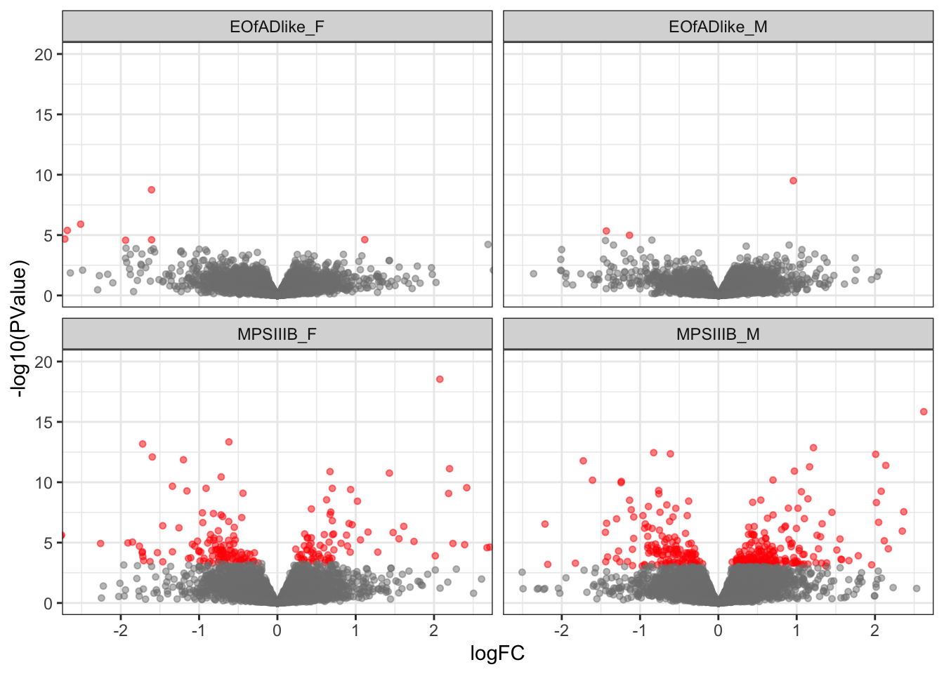

MD plot

toptables_cqn_bygroup %>%
  bind_rows() %>% 
  ggplot(aes(x = logCPM, y = logFC)) +
  geom_point(
    aes(colour = DE),
    alpha = 0.5
  ) +
  facet_wrap(~coef, ncol = 1) +
  theme(legend.position = "none") +
  scale_color_manual(values = c("grey50", "red")) +
  geom_smooth(se = F)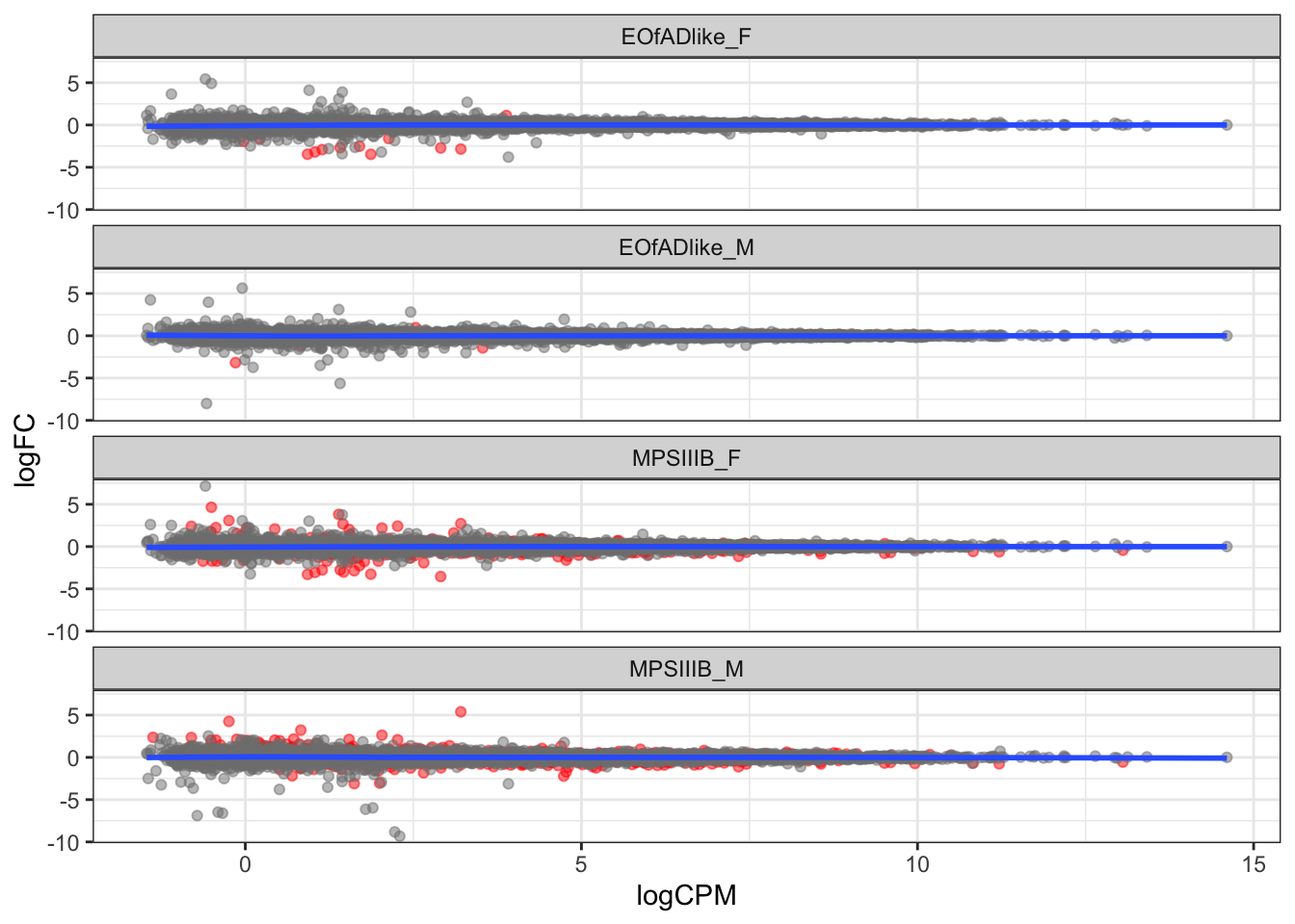

Gene set enrichment analysis

I now am going to test the KEGG, gene ontology (GO), iron-responsive element (IRE), cell type markers and chromosomal location gene sets to determine whether any of them display changes to gene expression as a group. The gene sets were obtained from MSIGDB using the msigdbr package.

Gene sets

The KEGG and GO terms were obtained from msigdb using msigdbr. These gene sets were filtered to only contain the genes above the detectable threshold in this experiment. Also, any gene sets with less than 5 genes were omitted, as these probably arent very biologically meaninigful. The GO terms were also restricted to those with 3 or more steps back to the ontology root terms.

The iron-responsive element (IRE) genes were obtained from Hin et al. 2021 (DOI: 10.3233/JAD-210200). The zebrafish IRE-containing genes were used, and were also filtered to only retain the detectable genes.

The chromosome gene sets were generated from the DGE object.

The cell type marker gene sets were obtained from the single-cell RNA-seq data of Jiang et al. 2021 (https://doi.org/10.3389/fcell.2021.743421)/

# Obtain the KEGG gene sets. 
KEGG <- msigdbr("Danio rerio", category = "C2", subcategory = "CP:KEGG") %>% 
  left_join(x$genes, by = c("gene_symbol" = "gene_name")) %>% 
  dplyr::filter(gene_id %in% rownames(x)) %>% 
  distinct(gs_name, gene_id, .keep_all = TRUE) %>% 
  split(f = .$gs_name) %>%
  lapply(extract2, "gene_id")

# calculate the number of genes per gene set
sizes <- KEGG %>% 
  lapply(length) %>% 
  unlist %>% 
  as.data.frame() %>% 
  set_colnames( "n_genes") %>% 
  rownames_to_column("gs")


# retain gene sets with at least 3 genes in it
KEGG <- KEGG[sizes %>% dplyr::filter(n_genes > 3) %>% .$gs]

# GO Terms summaries that The UofA biohub made. 
goSummaries <- url("https://uofabioinformaticshub.github.io/summaries2GO/data/goSummaries.RDS") %>%
  readRDS() %>%
  mutate(
    Term = Term(id),
    gs_name = Term %>% str_to_upper() %>% str_replace_all("[ -]", "_"),
    gs_name = paste0("GO_", gs_name)
    )

minPath <- 3

# obtain the GO terms 
GO <- 
  msigdbr("Danio rerio", category = "C5") %>% 
  dplyr::filter(grepl(gs_name, pattern = "^GO")) %>% 
  left_join(x$genes, by = c("gene_symbol" = "gene_name")) %>% 
  dplyr::filter(gene_id %in% rownames(x)) %>% 
  mutate(gs_name = str_replace(gs_name, pattern = "GOBP_", replacement = "GO_")) %>% 
  mutate(gs_name = str_replace(gs_name, pattern = "GOMF_", replacement = "GO_")) %>%     
  mutate(gs_name = str_replace(gs_name, pattern = "GOCC_", replacement = "GO_")) %>%     
  left_join(goSummaries) %>% 
  dplyr::filter(shortest_path >= minPath) %>%
  distinct(gs_name, gene_id, .keep_all = TRUE) %>% 
  split(f = .$gs_name) %>%
  lapply(extract2, "gene_id")

GOdf <-  msigdbr("Danio rerio", category = "C5") %>%
  dplyr::filter(grepl(gs_name, pattern = "^GO")) %>%
  left_join(x$genes, by = c("gene_symbol" = "gene_name")) %>%
  dplyr::filter(gene_id %in% rownames(x)) %>%
  mutate(
    gs_full_name = gs_name, 
    gs_name = str_replace(gs_name, pattern = "GOBP_", replacement = "GO_"), 
    gs_name = str_replace(gs_name, pattern = "GOMF_", replacement = "GO_"), 
    gs_name = str_replace(gs_name, pattern = "GOCC_", replacement = "GO_")
  ) %>%
  left_join(goSummaries) %>%
  dplyr::filter(shortest_path >= minPath) %>%
  distinct(gs_name, gene_id, .keep_all = TRUE) 

sizes_GO <- GO %>%
  lapply(length) %>%
  unlist %>%
  as.data.frame() %>%
  set_colnames( "n_genes") %>%
  rownames_to_column("gs")


# retain gene sets with at least 3 genes in it
GO <- GO[sizes_GO %>% dplyr::filter(n_genes > 3) %>% .$gs]

ireGenes <- readRDS("data/gene_sets/zebrafishireGenes.rds") %>% 
  unlist() %>% 
  as.data.frame() %>% 
  rownames_to_column("ire") %>% 
  as_tibble() %>% 
  mutate(ire = str_extract(ire, pattern = "ire[:digit:]_[:alpha:]+")) %>% 
  set_colnames(c("ire", "gene_id")) %>% 
  dplyr::filter(gene_id %in% rownames(x)) %>% 
  split(f = .$ire) %>% 
  lapply(magrittr::extract2,"gene_id") 

chr <- x$genes %>% 
  dplyr::select(gene_id, chromosome) %>% 
  split(f = .$chromosome) %>%
  lapply(extract2, "gene_id") %>% 
  .[c("MT", seq(1:25))] # omit the ALT chromosmes and scaffolds


cell_type_markers <- 
  read_xlsx("data/gene_sets/Suppdata2_jiangetal_2021_fcelldev.xlsx", sheet = "Brain") %>% 
  dplyr::rename("gene_name" = gene) %>% 
  left_join(x$genes) %>% 
  dplyr::filter(gene_id %in% rownames(x)) %>% 
  split(f = .$`cell type`) %>% 
  lapply(extract2, "gene_id")
  

cell_type_markers %<>% 
  lapply(function(y) {
    y[y %in% rownames(x)]
  })

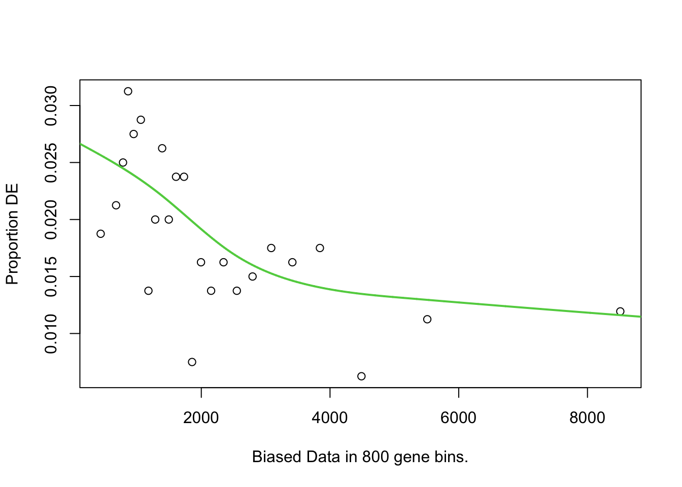
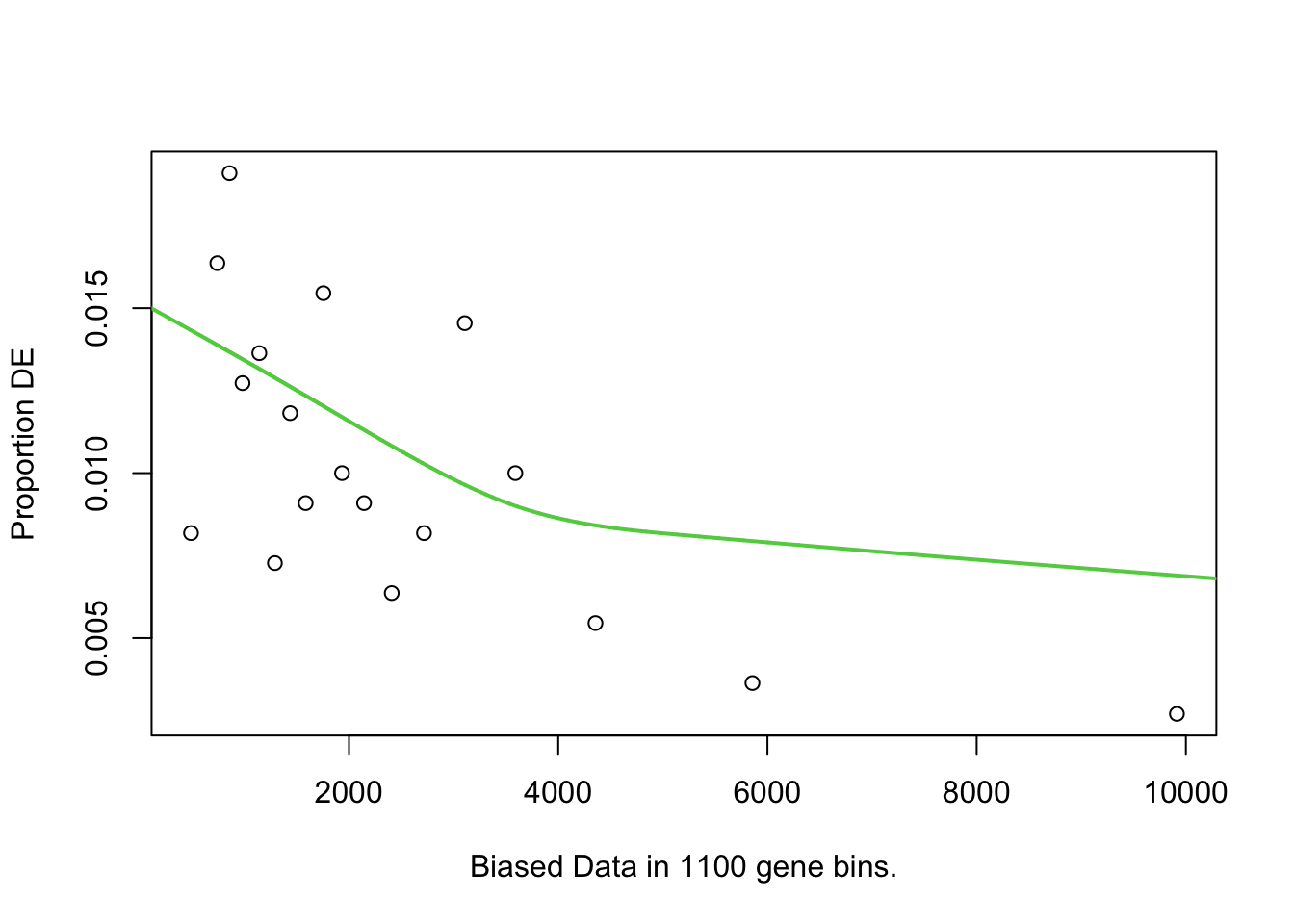
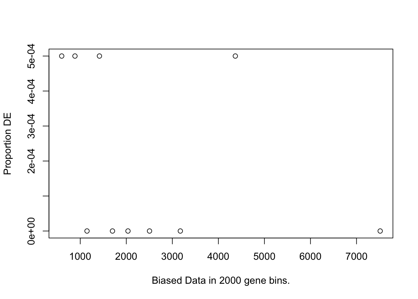
GOSEQ

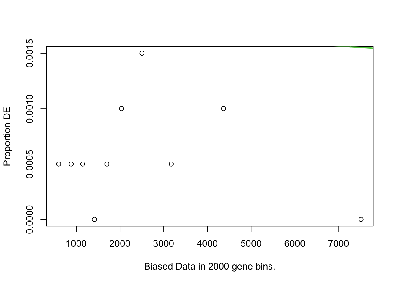
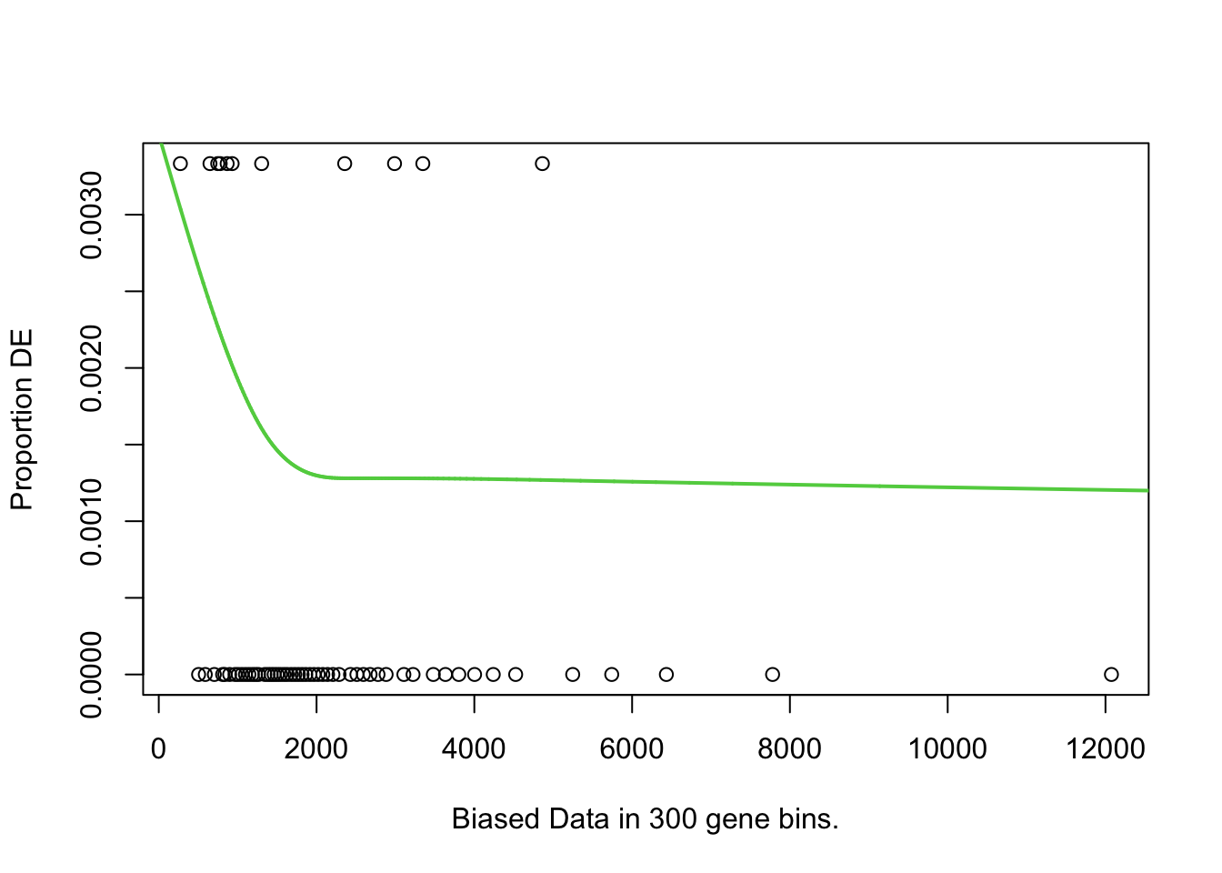
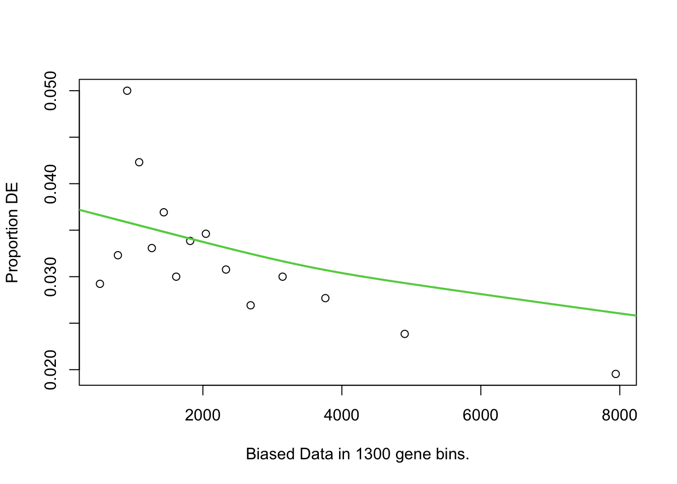
I first will look at enrichment of GO terms within the DE genes using goseq. I like goseq as it lets you include a covariate. Since there was still a bit of bias left after cqn for gene length, i will use this as the covariate.

pwfs <- 
  c(toptables_cqn_bygroup, toptables_cqn_simple) %>% 
  lapply(function(y) {
    
    y %>% 
      with(
        nullp(
          DEgenes = structure(DE, names = gene_id), 
          bias.data = length
        )
      )
  })

goseq.results <- 
  pwfs %>% 
  lapply(function(y) {
    goseq(y, gene2cat = GO) %>% 
      as_tibble() %>% 
      mutate(
        FDR = p.adjust(over_represented_pvalue, method = "fdr")
        ) %>% 
      dplyr::select(-under_represented_pvalue) %>% 
      left_join(GOdf %>% dplyr::select(category = gs_name, gs_subcat) %>% unique) %>% 
      dplyr::select(GO = category, GO_subcat = gs_subcat, everything())
  })

goseq.results %<>% 
  map2(names(.), ~.x %>% mutate(coef = .y))

HMP

Since I’m not detecting any significant gene sets in the EOfAD-like mutants, I need to try another method. I will use the harmonic mean p val method which combines indivisual p vals from 3 gene set enrichmen analysis methods: fry, camera and gsea.

# a function to run the HMP calculation. 
runHMP = function(
  geneset, 
  logCPM,
  toptable, 
  design, 
  contrasts
  
) {
 
  # run fry
  fry <- 
    colnames(contrasts) %>% 
  sapply(function(y) {
    logCPM %>%
      limma::fry(
        index = geneset,
        design = design,
        contrast = contrasts[,y],
        sort = "mixed"
      ) %>%
      rownames_to_column("pathway") %>%
      as_tibble() %>% 
      mutate(
        coef = y, 
        coef = str_remove(coef, pattern = " - wt.+")
        ) 
  }, simplify = FALSE)

  # run camera
  camera <- colnames(contrasts) %>% 
  sapply(function(y) {
    logCPM %>%
      limma::camera(
        index = geneset,
        design = design,
        contrast = contrasts[,y]
      ) %>%
      rownames_to_column("pathway") %>%
      as_tibble() %>% 
      mutate(coef = y, 
             coef = str_remove(coef, pattern = " - wt.+")) 
  }, simplify = FALSE)
  
  # create ranks for fgsea
  ranks <-
    sapply(toptable, function(y) {
      y %>%
        mutate(rankstat = sign(logFC) * log10(1/PValue)) %>%
        arrange(rankstat) %>%
        dplyr::select(c("gene_id", "rankstat")) %>% #only want the Pvalue with sign
        with(structure(rankstat, names = gene_id)) %>%
        rev() # reverse so the start of the list is upregulated genes
    }, simplify = FALSE)
  
  # run fgsea
  set.seed(1)
  fgsea <- ranks %>% 
  sapply(function(x){
    fgseaMultilevel(stats = x, 
                    pathways = geneset) %>%
      as_tibble() %>%
      dplyr::rename(FDR = padj) %>%
      mutate(padj = p.adjust(pval, "bonferroni")) %>%
      dplyr::select(pathway, pval, FDR, padj, everything()) %>%
      arrange(pval) 
  }, simplify = F)
  
  fgsea %<>% 
    map2(names(.), ~.x %>% mutate(coef = .y))  

  
  # calculate HMP
  hmp <- 
    fry %>%
    bind_rows() %>%
    dplyr::select(pathway, PValue.Mixed, coef) %>%
    dplyr::rename(fry_p = PValue.Mixed) %>%
    left_join(camera %>%
                bind_rows() %>%
                dplyr::select(pathway, PValue, coef),
              by = c("pathway", "coef")) %>%
    dplyr::rename(camera_p = PValue) %>%
    left_join(fgsea %>%
                bind_rows() %>%
                dplyr::select(pathway, pval, coef),
              by = c("pathway", "coef")) %>%
    dplyr::rename(fgsea_p = pval) %>%
    bind_rows() %>%
    nest(p = one_of(c("fry_p", "camera_p", "fgsea_p"))) %>%
    mutate(harmonic_p = vapply(p, function(x){
      x <- unlist(x)
      x <- x[!is.na(x)]
      p.hmp(x, L = 4)
    }, numeric(1))
    ) %>%
    unnest() %>%
    mutate(harmonic_p_FDR = p.adjust(harmonic_p, "fdr"),
           sig = harmonic_p_FDR < 0.05) %>%
    arrange(harmonic_p)
  
  return( 
    list(
      hmp = hmp,
      fgsea = fgsea
    ))
}

KEGG

hmp.adult.kegg.cqn.bygroup <- runHMP(
  geneset = KEGG, logCPM = logCPM, 
  toptable = toptables_cqn_bygroup, 
  design = design.bygroup, contrasts = contrasts
  )

sig.kegg.morethan1 <- hmp.adult.kegg.cqn.bygroup$hmp %>% 
  dplyr::filter(harmonic_p_FDR < 0.05) %>% 
  group_by(pathway) %>% 
  summarise(n = n()) %>% 
  ungroup %>% 
  dplyr::filter(n > 1)

hmp.adult.kegg.cqn.bygroup$hmp %>%   
  dplyr::filter(pathway %in% sig.kegg.morethan1$pathway) %>% 
  left_join(sig.kegg.morethan1) %>% 
  mutate(
    sex = case_when(
      grepl(coef, pattern = "_F") ~ "female", 
      grepl(coef, pattern = "_M") ~ "male"
    )
  ) %>% 
  ggplot(
    aes(
      x = coef, 
      y = reorder(pathway, n-harmonic_p)
      )) +
  geom_tile(
    aes(fill = -log10(harmonic_p), alpha = sig)
  ) +
  geom_label(
    aes(label = signif(harmonic_p_FDR, 2))
  ) +
  scale_fill_viridis_c() +
  facet_wrap(~sex, scales = "free_x")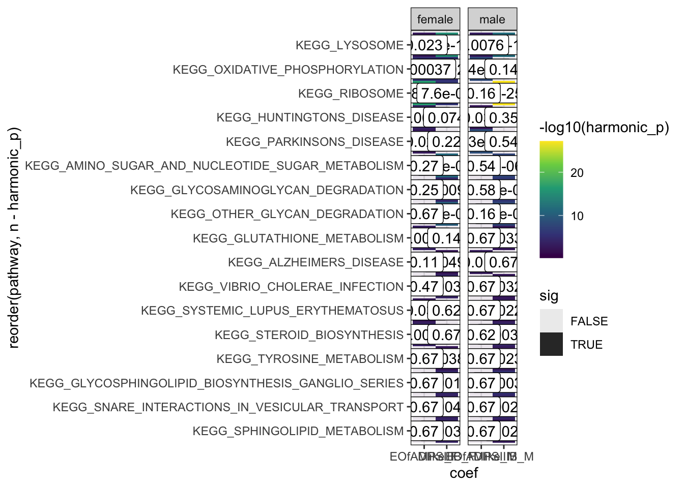

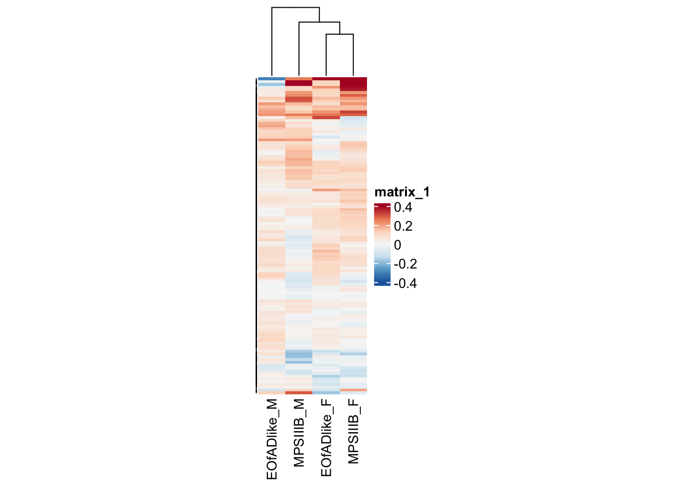
oxidative phosphorylation

oxphos.adult <- toptables_cqn_bygroup %>% 
  bind_rows() %>% 
  dplyr::filter(gene_id %in% KEGG$KEGG_OXIDATIVE_PHOSPHORYLATION) %>% 
  dplyr::select(gene_name, logFC, coef) %>% 
  dplyr::distinct(gene_name, coef, .keep_all = T) %>% 
  spread(key = "coef", value = "logFC") %>% 
  column_to_rownames("gene_name") %>% 
  as.matrix()

#png("output/plots/new_KEGG_hms/oxphos.png", width = 8, height = 12, units = "cm", res = 300)
pheatmap(
  oxphos.adult, 
  color = colorRampPalette(rev(brewer.pal(n = 7, name = "RdBu")))(100), 
  breaks = seq(-0.4,0.4, by = 0.01), 
  cellwidth = 20, 
  treeheight_row = 0, 
  show_rownames = FALSE
  )

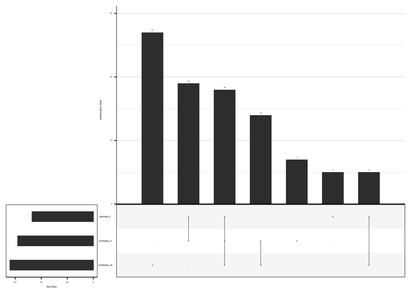
#dev.off()

upset plot to show the overlap of leading edge genes

#png("output/plots/new_KEGG_hms/oxphos_upset.png", width = 3.5, height = 3.5, units = "cm", res = 300)
hmp.adult.kegg.cqn.bygroup$fgsea %>% 
  bind_rows() %>% 
  dplyr::filter(coef != "MPSIIIB_M") %>% 
  dplyr::filter(pathway == "KEGG_OXIDATIVE_PHOSPHORYLATION") %>% 
  dplyr::select(coef, leadingEdge) %>% 
  split(f = .$coef) %>% 
  lapply(function(y) {y$leadingEdge[[1]]}) %>% 
  fromList() %>% 
  upset(
    order.by = "freq", 
    #mb.ratio = c(0.5,0.5),
    text.scale = 0.4, 
    point.size = 0.2,
    line.size = 0.2, 
    set_size.show = FALSE
  )

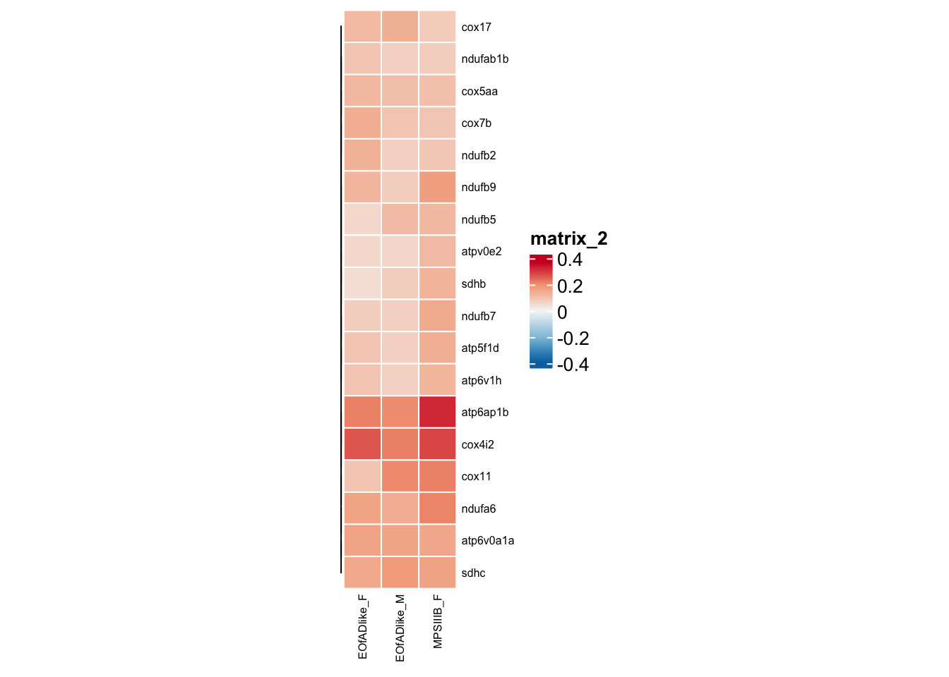
#dev.off()

shared leading edge genes:

leadingedge.oxphos <- hmp.adult.kegg.cqn.bygroup$fgsea %>% 
  bind_rows() %>% 
  dplyr::filter(pathway == "KEGG_OXIDATIVE_PHOSPHORYLATION") %>% 
  dplyr::filter(coef != "MPSIIIB_M") %>% 
  dplyr::select(coef, leadingEdge) %>% 
  split(f = .$coef) %>% 
  lapply(function(y) {y$leadingEdge[[1]]}) 


#png("output/plots/new_KEGG_hms/oxphos_leadingedge.png", width = 8, height = 6, units = "cm", res = 300)
toptables_cqn_bygroup %>% 
  bind_rows() %>% 
  dplyr::filter(gene_id %in% Reduce(intersect, leadingedge.oxphos)) %>% 
  dplyr::select(gene_name, logFC, coef) %>% 
  dplyr::filter(coef != "MPSIIIB_M") %>% 
  dplyr::distinct(gene_name, coef, .keep_all = T) %>% 
  spread(key = "coef", value = "logFC") %>% 
  column_to_rownames("gene_name") %>% 
  as.matrix() %>% 
  pheatmap(
    color = colorRampPalette(rev(brewer.pal(n = 5, name = "RdBu")))(100), 
    breaks = seq(-0.4, 0.4, by = 0.1), 
    cluster_cols = F, 
    cellwidth = 20,
    treeheight_row = 0, 
    fontsize = 6, 
    border_color = "white", 
    height = 20
  )

#dev.off()

lysosome

lyso.adult <- toptables_cqn_bygroup %>% 
  bind_rows() %>% 
  dplyr::filter(gene_id %in% KEGG$KEGG_LYSOSOME) %>% 
  dplyr::select(gene_name, logFC, coef) %>% 
  dplyr::distinct(gene_name, coef, .keep_all = T) %>% 
  spread(key = "coef", value = "logFC") %>% 
  column_to_rownames("gene_name") %>% 
  as.matrix()

#png("output/plots/new_KEGG_hms/lyso.png", width = 8, height = 12, units = "cm", res = 300)
pheatmap(
  lyso.adult, 
  color = colorRampPalette(rev(brewer.pal(n = 7, name = "RdBu")))(100), 
  breaks = seq(-0.5,0.5, by = 0.01), 
  cellwidth = 20, 
  treeheight_row = 0, 
  show_rownames = FALSE
  )

#dev.off()

upset plot to show the overlap of leading edge genes

#png("output/plots/new_KEGG_hms/lyso_upset.png", width = 3.5, height = 3.5, units = "cm", res = 300)
hmp.adult.kegg.cqn.bygroup$fgsea %>% 
  bind_rows() %>% 
  dplyr::filter(pathway == "KEGG_LYSOSOME") %>% 
  dplyr::select(coef, leadingEdge) %>% 
  split(f = .$coef) %>% 
  lapply(function(y) {y$leadingEdge[[1]]}) %>%
  fromList() %>% 
  upset(
    order.by = "freq", 
    #mb.ratio = c(0.5,0.5),
    text.scale = 0.4, 
    point.size = 0.2,
    line.size = 0.2, 
    set_size.show = FALSE
  )

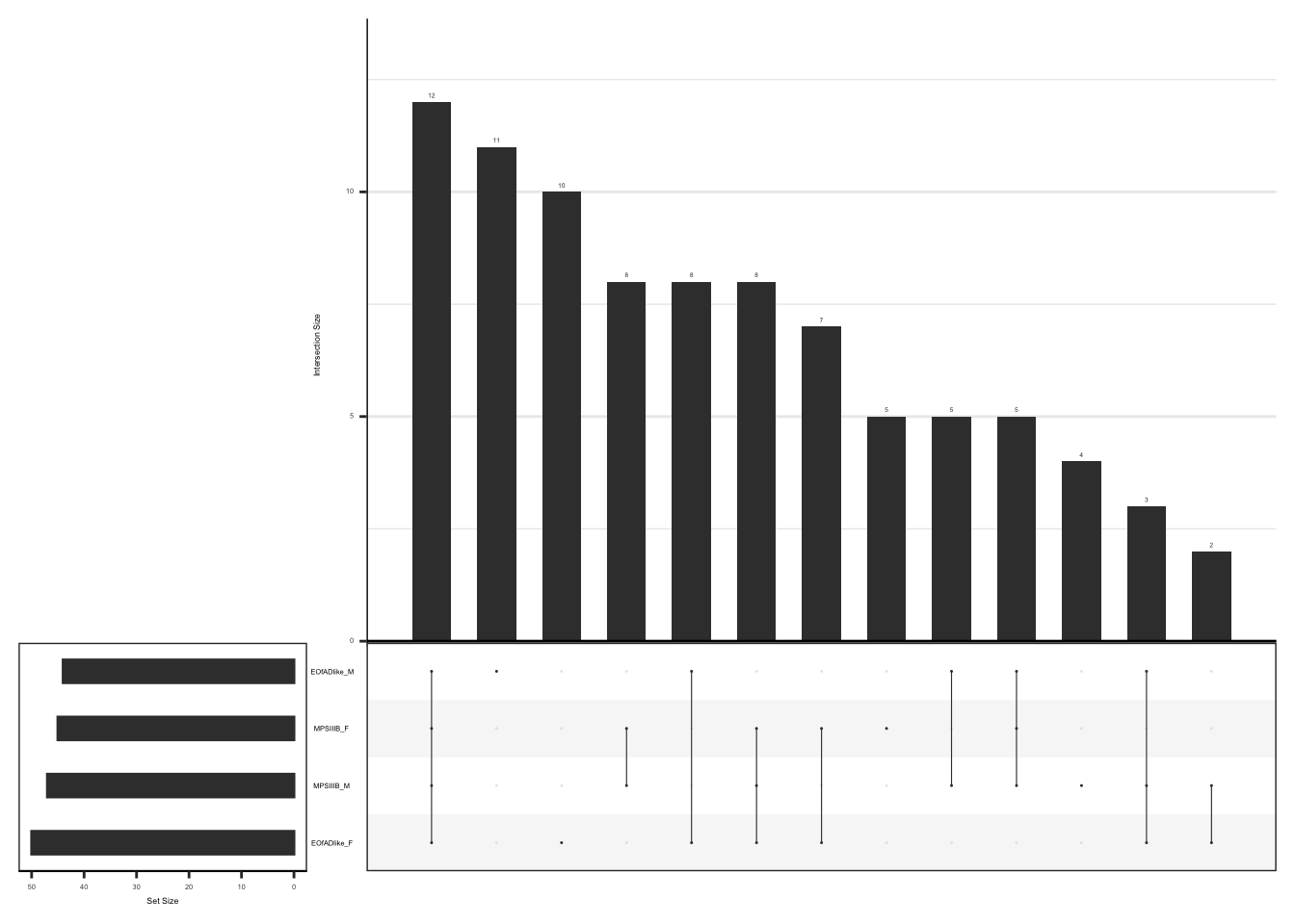
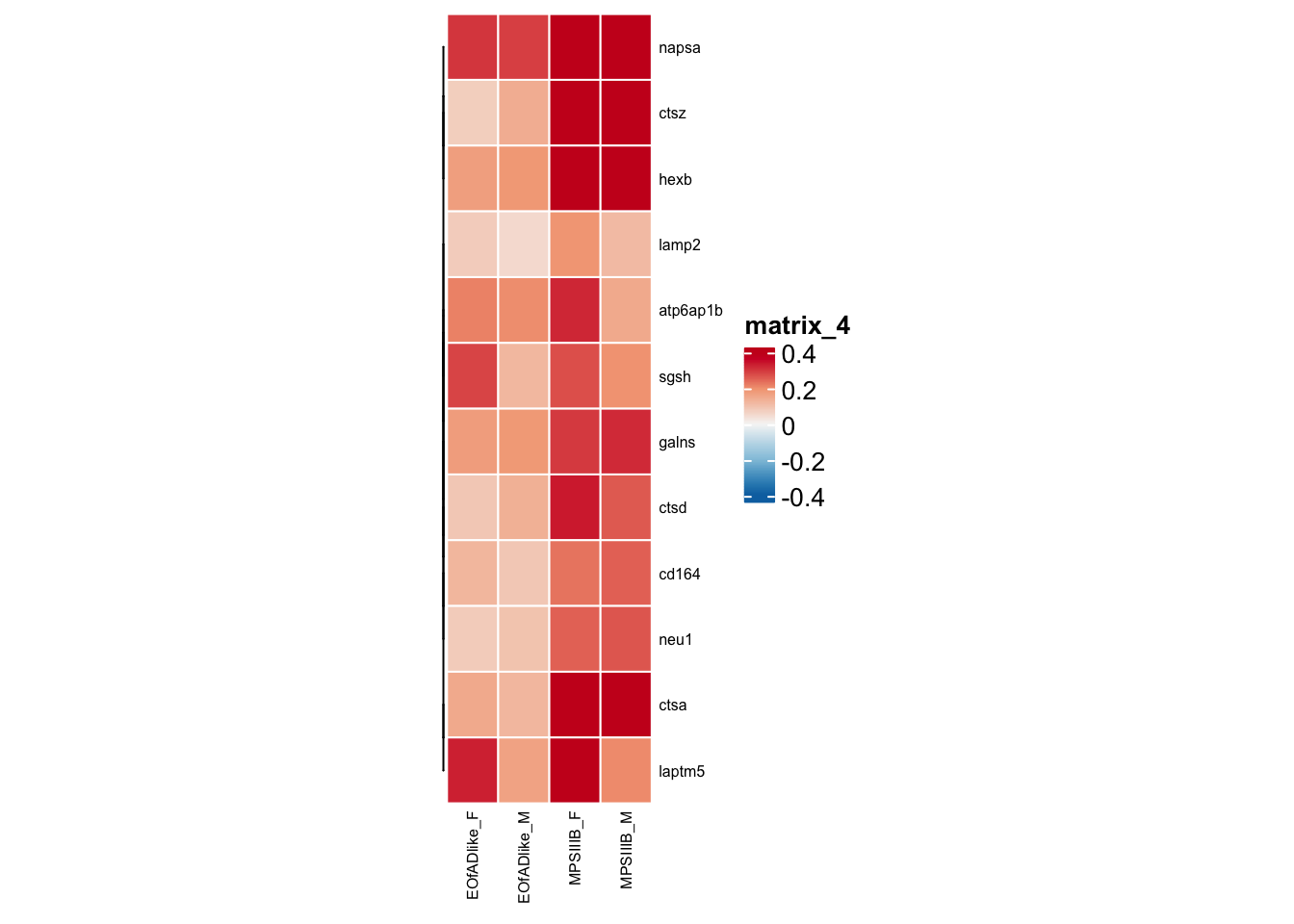
#dev.off()

leading edge genes shared

leadingedge.lyso <- hmp.adult.kegg.cqn.bygroup$fgsea %>% 
  bind_rows() %>% 
  dplyr::filter(pathway == "KEGG_LYSOSOME") %>% 
  dplyr::select(coef, leadingEdge) %>% 
  split(f = .$coef) %>% 
  lapply(function(y) {y$leadingEdge[[1]]}) 

#png("output/plots/new_KEGG_hms/lyso_leadingedge.png", width = 8, height = 6, units = "cm", res = 300)
toptables_cqn_bygroup %>% 
  bind_rows() %>% 
  dplyr::filter(gene_id %in% Reduce(intersect, leadingedge.lyso)) %>% 
  dplyr::select(gene_name, logFC, coef) %>% 
  dplyr::distinct(gene_name, coef, .keep_all = T) %>% 
  spread(key = "coef", value = "logFC") %>% 
  column_to_rownames("gene_name") %>% 
  as.matrix() %>% 
  pheatmap(
    color = colorRampPalette(rev(brewer.pal(n = 5, name = "RdBu")))(100), 
    breaks = seq(-0.4, 0.4, by = 0.1), 
    cluster_cols = F, 
    cellwidth = 20,
    treeheight_row = 0, 
    fontsize = 6, 
    border_color = "white", 
    height = 20
  )

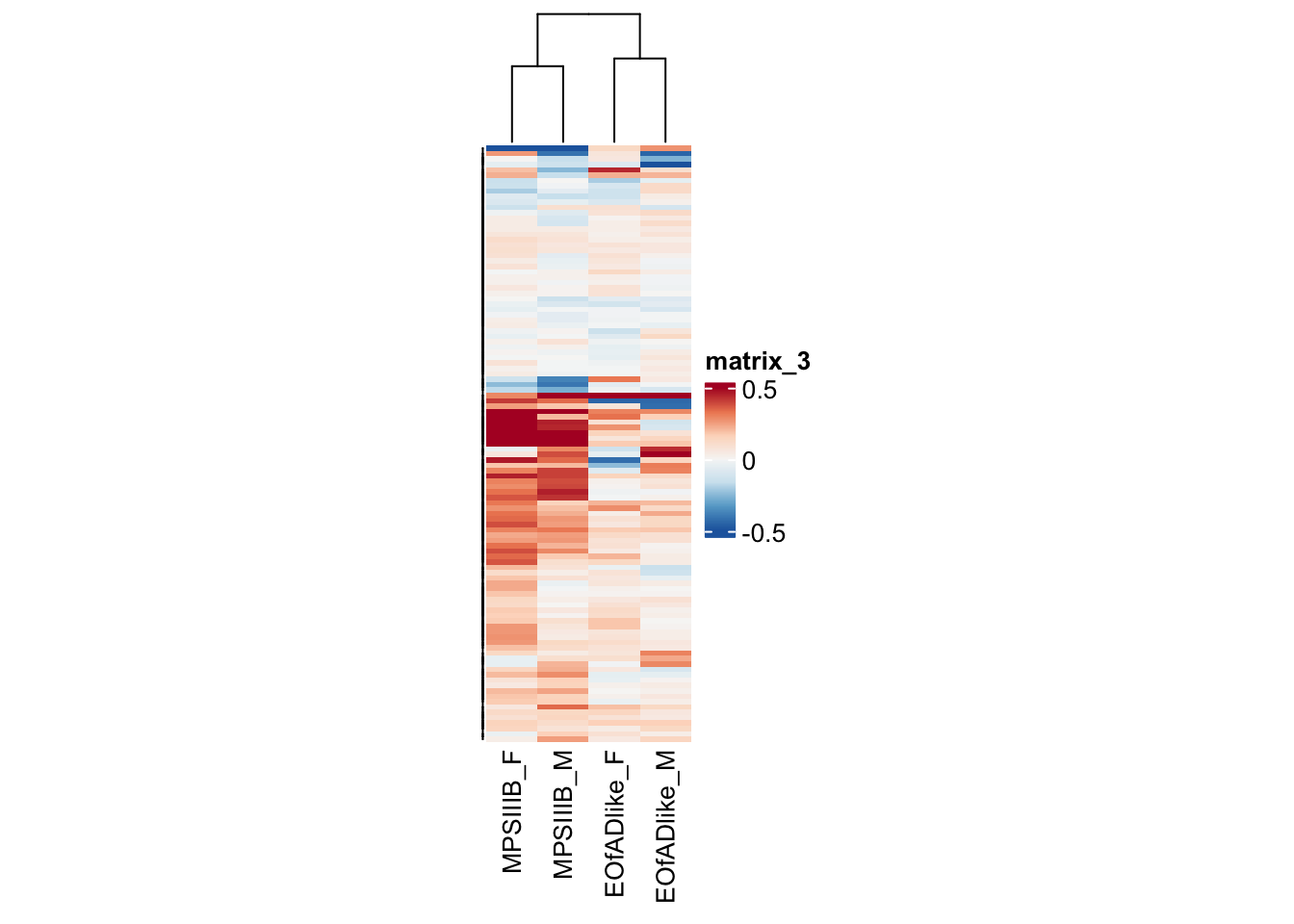
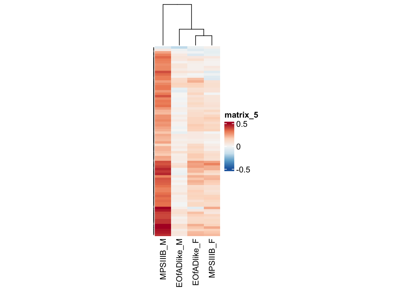
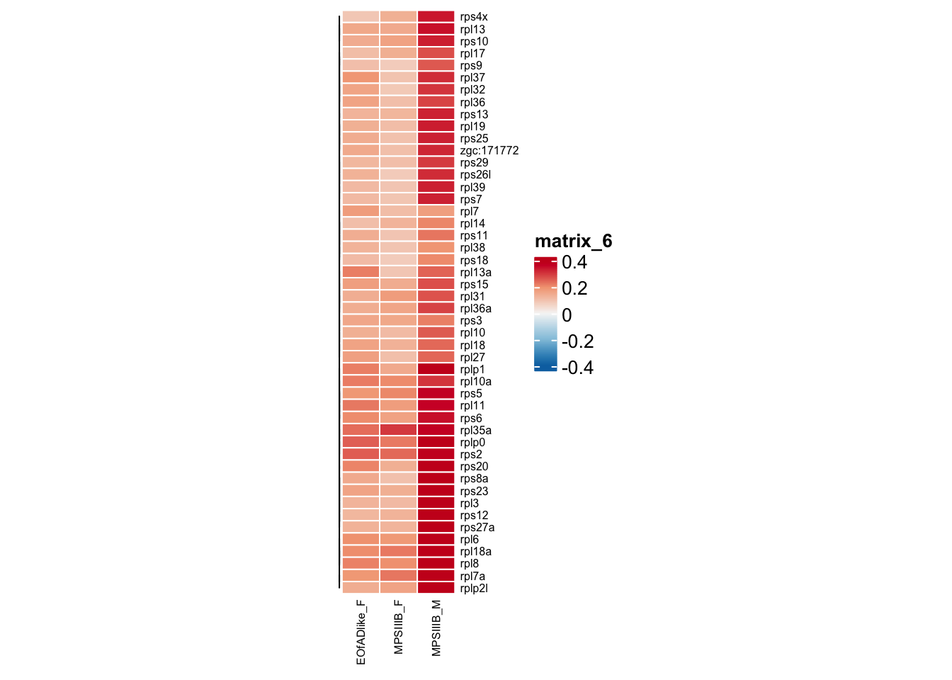
#dev.off()

ribosome

ribo.adult <- toptables_cqn_bygroup %>% 
  bind_rows() %>% 
  dplyr::filter(gene_id %in% KEGG$KEGG_RIBOSOME) %>% 
  dplyr::select(gene_name, logFC, coef) %>% 
  dplyr::distinct(gene_name, coef, .keep_all = T) %>% 
  spread(key = "coef", value = "logFC") %>% 
  column_to_rownames("gene_name") %>% 
  as.matrix()

#png("output/plots/new_KEGG_hms/ribo.png", width = 8, height = 12, units = "cm", res = 300)
pheatmap(
  ribo.adult, 
  color = colorRampPalette(rev(brewer.pal(n = 7, name = "RdBu")))(100), 
  breaks = seq(-0.5,0.5, by = 0.01), 
  cellwidth = 20, 
  treeheight_row = 0, 
  show_rownames = FALSE, 
  border_color = NA
  )

#dev.off()

upset plot to show the overlap of leading edge genes

# png("output/plots/new_KEGG_hms/ribo_upset.png", width = 3.5, height = 3.5, units = "cm", res = 300)
hmp.adult.kegg.cqn.bygroup$fgsea %>% 
  bind_rows() %>% 
  dplyr::filter(pathway == "KEGG_RIBOSOME") %>% 
  dplyr::filter(coef != "EOfADlike_M") %>% 
  dplyr::select(coef, leadingEdge) %>% 
  split(f = .$coef) %>% 
  lapply(function(y) {y$leadingEdge[[1]]}) %>%
  fromList() %>% 
  upset(
    order.by = "freq", 
    #mb.ratio = c(0.5,0.5),
    text.scale = 0.4, 
    point.size = 0.2,
    line.size = 0.2, 
    set_size.show = FALSE
  )

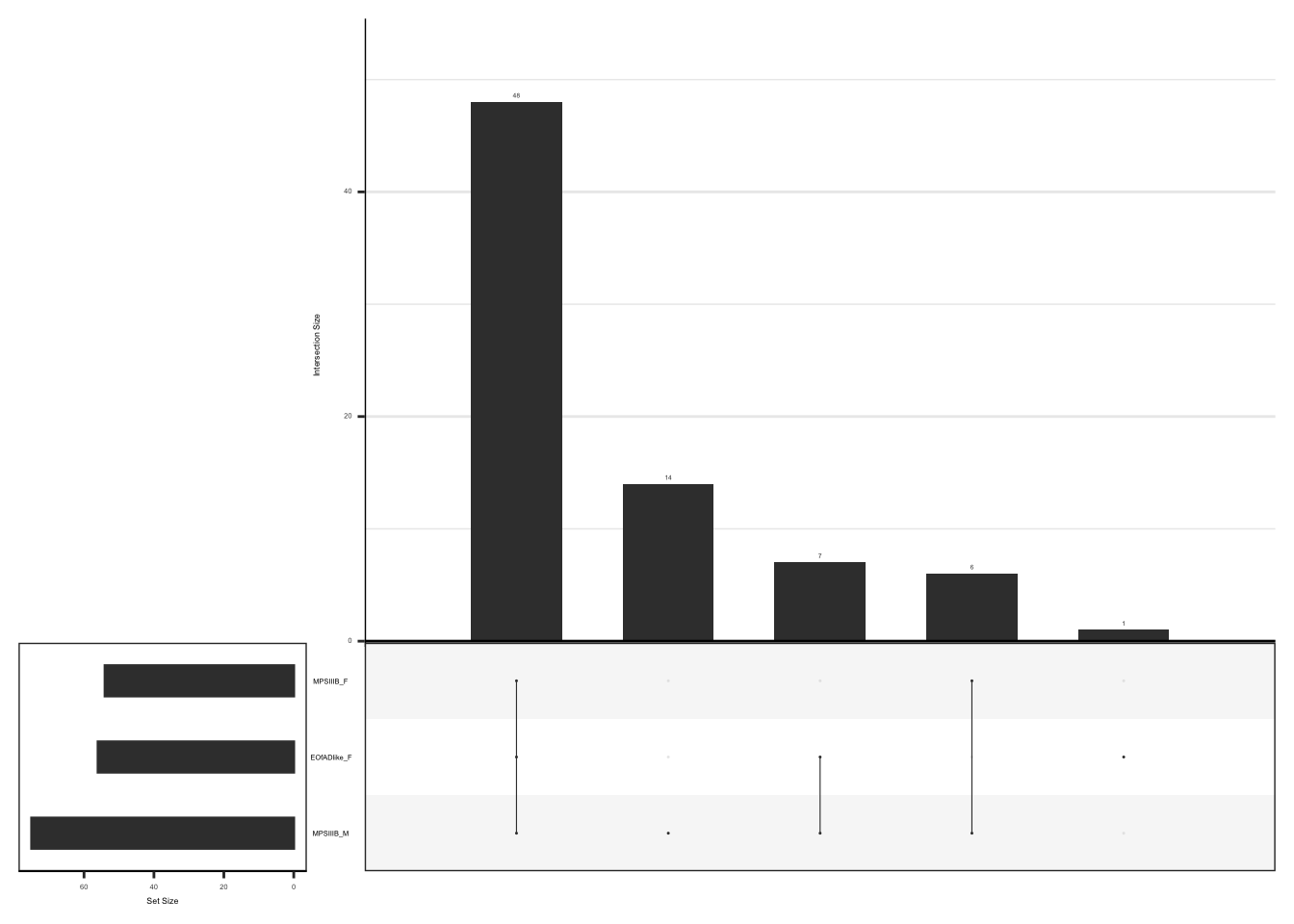
#dev.off()

shared leadging edge genes

leadingedge.ribo <- hmp.adult.kegg.cqn.bygroup$fgsea %>% 
  bind_rows() %>% 
  dplyr::filter(pathway == "KEGG_RIBOSOME") %>% 
  dplyr::filter(coef != "EOfADlike_M") %>% 
  dplyr::select(coef, leadingEdge) %>% 
  split(f = .$coef) %>% 
  lapply(function(y) {y$leadingEdge[[1]]}) 

#png("output/plots/new_KEGG_hms/ribo_leadingedge.png", width = 8, height = 10, units = "cm", res = 300)
toptables_cqn_bygroup %>% 
  bind_rows() %>% 
  dplyr::filter(coef != "EOfADlike_M") %>% 
  dplyr::filter(gene_id %in% Reduce(intersect, leadingedge.ribo)) %>% 
  dplyr::select(gene_name, logFC, coef) %>% 
  dplyr::distinct(gene_name, coef, .keep_all = T) %>% 
  spread(key = "coef", value = "logFC") %>% 
  column_to_rownames("gene_name") %>% 
  as.matrix() %>% 
  pheatmap(
    color = colorRampPalette(rev(brewer.pal(n = 5, name = "RdBu")))(100), 
    breaks = seq(-0.4, 0.4, by = 0.1), 
    cluster_cols = F, 
    cellwidth = 20,
    treeheight_row = 0, 
    fontsize = 6, 
    border_color = "white", 
    height = 22
  )

#dev.off()

inflammation gene sets

plot.cell.type.hm = function(celltype.gs, plot.title) {

  toptables_cqn_bygroup %>%
    bind_rows() %>%
    mutate(
      exp = "mRNA"
    ) %>%
    dplyr::select(
      gene_name, logFC, PValue, FDR, coef, exp
    ) %>%
    bind_rows(
      toptables %>%
        bind_rows() %>%
        mutate(exp = "protein") %>%
        dplyr::filter(coef != "wt_M - wt_F") %>%
        dplyr::select(
          gene_name, logFC, PValue = pval, FDR, coef, exp
        )
    ) %>%
    dplyr::filter(
      gene_name %in% celltype.gs
    ) %>%
    group_by(exp) %>%

    tidyHeatmap::heatmap(
      # input data
      .column = gene_name,
      .row = coef,
      .value = logFC,

      # colours
      palette_value = circlize::colorRamp2(
        seq(-0.4, 0.4, length.out = 11),
        rev(RColorBrewer::brewer.pal(11, "RdBu"))),
      rect_gp = grid::gpar(col = "#161616", lwd = 0.5),

      # sizes
      row_names_gp = gpar(fontsize = 14),
      column_names_gp = gpar(fontsize = 14),
      heatmap_width = unit(28, "cm"),
      heatmap_height = unit(11, "cm"),

      # dendro
      cluster_rows = FALSE,
      show_column_dend = F,
      show_row_dend = F
    ) %>%
    annotation_tile(exp, show_legend = FALSE) %>%
    wrap_heatmap() +
    ggtitle(label = paste(plot.title))

}

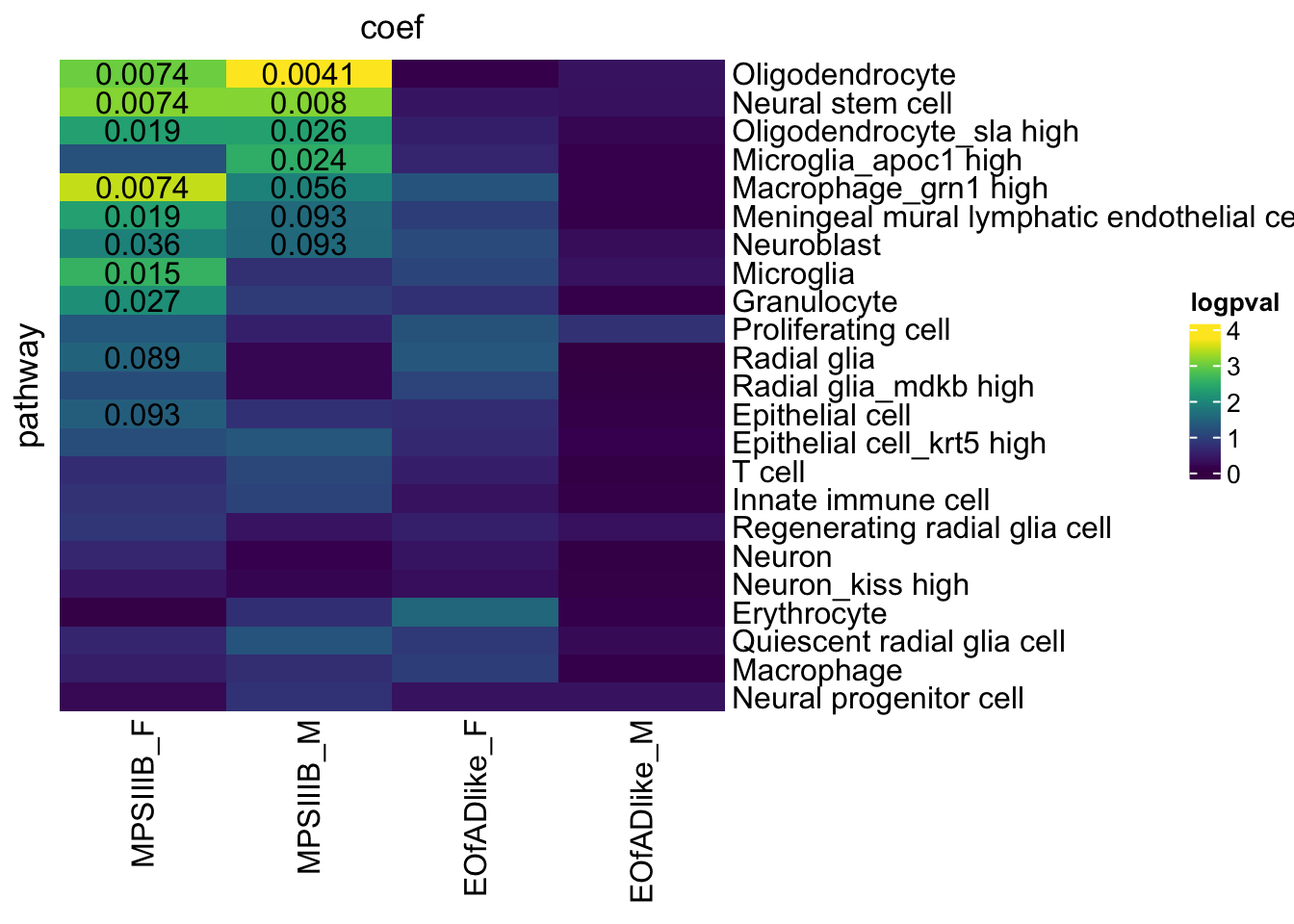
fry: cell types

fry.celltype.RNAseq <- 
  colnames(contrasts) %>% 
  sapply(function(y) {
    logCPM %>%
      limma::fry(
        index = cell_type_markers,
        design = design.bygroup,
        contrast = contrasts[,y],
        sort = "directional"
      ) %>%
      rownames_to_column("pathway") %>%
      as_tibble() %>% 
      mutate(
        coef = y, 
        coef = str_remove(coef, pattern = " - wt.+") # cleanup the coef col
      ) 
  }, simplify = FALSE)


fry.celltype.RNAseq %>% 
  bind_rows() %>% 
  mutate(
    logpval = -log10(PValue), 
    FDR = signif(FDR, 2)
    ) %>% 
  tidyHeatmap::heatmap(
    
    .row = pathway, 
    .column = coef, 
    .value = logpval, 
    
    show_column_dend = F,
    show_row_dend = F,
    
    col = viridis::viridis(30)
  
) %>% 
  layer_text(
    .value = FDR, 
    FDR < 0.1
    )

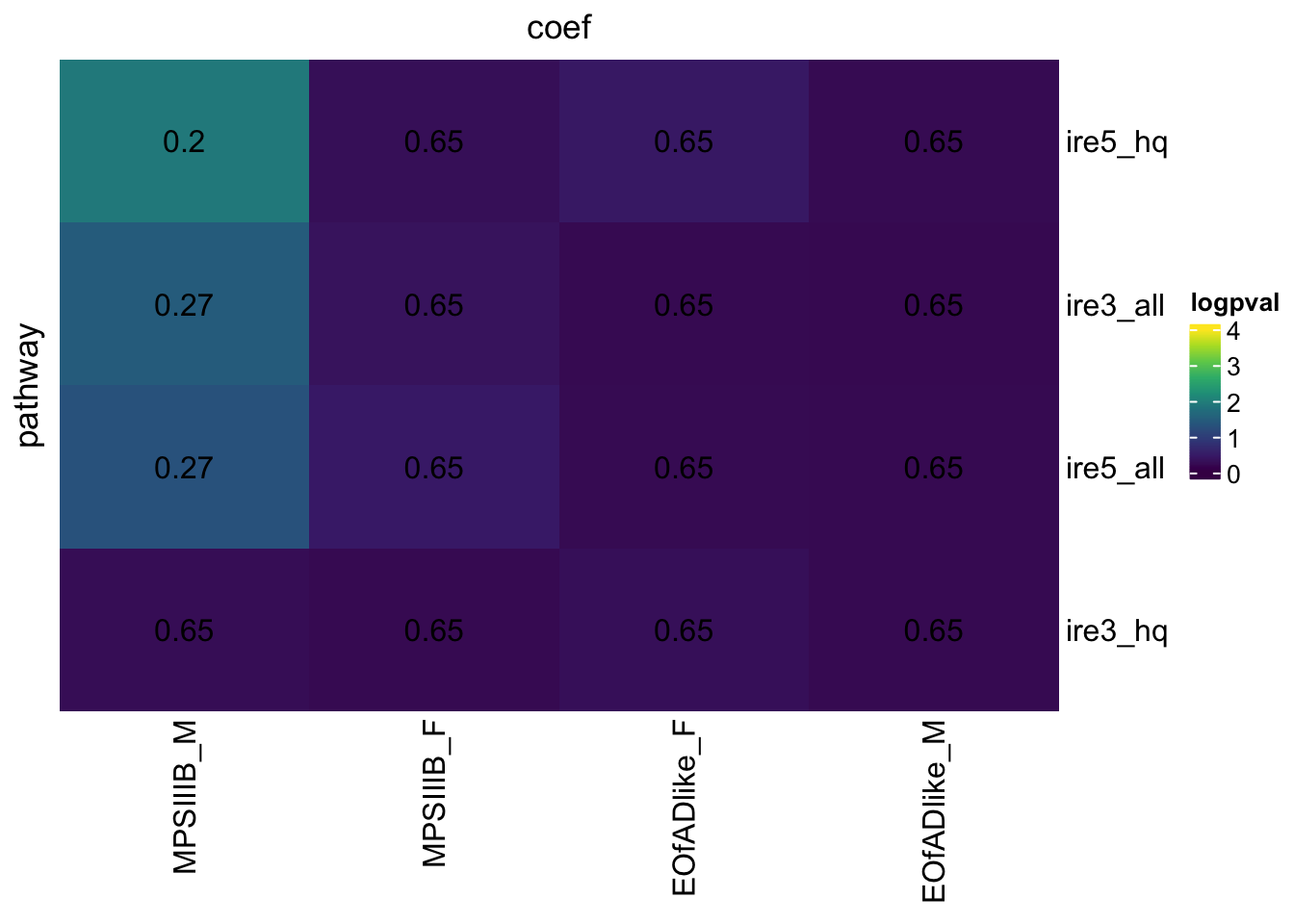
HMP IRE

hmp.adult.IREgenes.cqn.bygroup <- runHMP(
  geneset = ireGenes, logCPM = logCPM, 
  toptable = toptables_cqn_bygroup, 
  design = design.bygroup, contrasts = contrasts
  )

hmp.adult.IREgenes.cqn.bygroup$hmp %>% 
  mutate(
    logpval = -log10(harmonic_p), 
    harmonic_p_FDR = signif(harmonic_p_FDR, 2)
    ) %>% 
  tidyHeatmap::heatmap(
    
    .row = pathway, 
    .column = coef, 
    .value = logpval, 
    
    show_column_dend = F,
    show_row_dend = F,
    
    col = colorRamp2(seq(0, 4, length = 10), viridis::viridis(10))
  ) %>% 
  layer_text(
    .value = harmonic_p_FDR,
    )

Post-hoc power calc

set.seed(2016)

# convert CQN logCPM to counts. 
mu <- logCPM %>% 
  as.data.frame() %>% 
  rownames_to_column("gene_id") %>% 
  gather(key = "sample", value = "logCPM", colnames(x)) %>%
  dplyr::filter(grepl(sample, pattern = "wt")) %>% 
  left_join(
    x$samples %>% dplyr::select(sample, lib.size)
    ) %>% 
  mutate(
    CPM = 10^logCPM, 
    counts = CPM * lib.size
    ) %>% 
  as_tibble() %>% 
  dplyr::select(-logCPM, - lib.size, -CPM) %>% 
  pivot_wider(
    names_from = "sample", values_from = "counts") %>% 
  column_to_rownames("gene_id") %>% 
  rowMeans()


disp <- logCPM %>% 
  as.data.frame() %>% 
  rownames_to_column("gene_id") %>% 
  gather(key = "sample", value = "logCPM", colnames(x)) %>%
  dplyr::filter(grepl(sample, pattern = "wt")) %>% 
  left_join(
    x$samples %>% dplyr::select(sample, lib.size)
    ) %>% 
  mutate(
    CPM = 10^logCPM, 
    counts = CPM * lib.size
    ) %>% 
  as_tibble() %>% 
  dplyr::select(-logCPM, - lib.size, -CPM) %>% 
  pivot_wider(
    names_from = "sample", values_from = "counts") %>% 
  column_to_rownames("gene_id") %>% 
  DGEList() %>% 
  estimateDisp() %>% 
  .$tagwise.dispersion

fc <- function(y){exp(rnorm(y, log(1), 0.5*log(2)))}

power <- ssizeRNA_vary(nGenes = dim(x)[1], # Num detectable genes
              pi0 = 0.9, # Proportion of non-DE genes
              m = 50, # pseudo sample size
              mu = mu, # Average read count for each gene in control group. Calculated from this current dataset)
              disp = disp, # Dispersion parameter for each gene
              fc = fc, # Fold change per gene
              fdr = 0.05, # FDR level to control
              power = 0.9, # power level
              maxN = 40,
              replace = T
                )

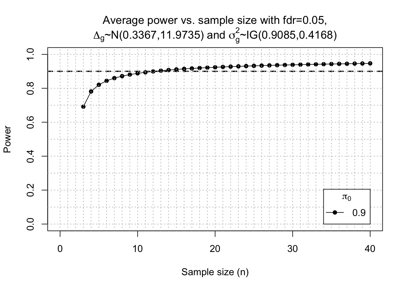
power$power %>% 
  as_tibble() %>% 
  set_colnames(c("n", "Power")) %>% 
  ggplot(aes(x = n, y = Power)) +
  geom_point() + 
  geom_line() +
  scale_x_continuous(limits = c(0,20))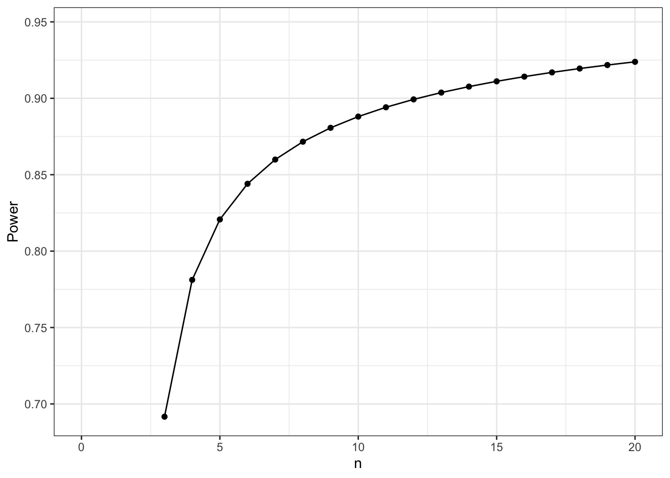

Data export

x %>% saveRDS("data/R_objects/adult_brain/dge.rds")
logCPM %>% saveRDS("data/R_objects/adult_brain/logcpm.rds")
toptables_cqn_bygroup %>% saveRDS("data/R_objects/adult_brain/toptablescqn_bysex.rds")
fry.celltype.RNAseq %>% saveRDS("data/R_objects/adult_brain/fry_cell_RNAseq.rds")
hmp.adult.IREgenes.cqn.bygroup %>% saveRDS("data/R_objects/adult_brain/hmp_ire.rds")
hmp.adult.kegg.cqn.bygroup %>% saveRDS("data/R_objects/adult_brain/hmp.kegg.rna.rds")

sessionInfo()

R version 4.3.2 (2023-10-31)
Platform: aarch64-apple-darwin20 (64-bit)
Running under: macOS Sonoma 14.3

Matrix products: default
BLAS:   /Library/Frameworks/R.framework/Versions/4.3-arm64/Resources/lib/libRblas.0.dylib 
LAPACK: /Library/Frameworks/R.framework/Versions/4.3-arm64/Resources/lib/libRlapack.dylib;  LAPACK version 3.11.0

locale:
[1] en_US.UTF-8/en_US.UTF-8/en_US.UTF-8/C/en_US.UTF-8/en_US.UTF-8

time zone: Australia/Adelaide
tzcode source: internal

attached base packages:
 [1] stats4    splines   grid      stats     graphics  grDevices utils    
 [8] datasets  methods   base     

other attached packages:
 [1] ensembldb_2.26.0        AnnotationFilter_1.26.0 GenomicFeatures_1.54.4 
 [4] AnnotationDbi_1.64.1    Biobase_2.62.0          GenomicRanges_1.54.1   
 [7] GenomeInfoDb_1.38.8     IRanges_2.36.0          S4Vectors_0.40.2       
[10] ssizeRNA_1.3.2          harmonicmeanp_3.0.1     FMStable_0.1-4         
[13] kableExtra_1.4.0        cqn_1.48.0              quantreg_5.97          
[16] SparseM_1.81            preprocessCore_1.64.0   nor1mix_1.3-3          
[19] mclust_6.1              fgsea_1.28.0            goseq_1.54.0           
[22] geneLenDataBase_1.38.0  BiasedUrn_2.0.11        edgeR_4.0.16           
[25] limma_3.58.1            UpSetR_1.4.0            circlize_0.4.16        
[28] tidyHeatmap_1.10.2      ComplexHeatmap_2.18.0   RColorBrewer_1.1-3     
[31] ggfortify_0.4.16        ggrepel_0.9.5           msigdbr_7.5.1          
[34] ggpubr_0.6.0            pheatmap_1.0.12         scales_1.3.0           
[37] pander_0.6.5            AnnotationHub_3.10.1    BiocFileCache_2.10.2   
[40] dbplyr_2.5.0            ngsReports_2.4.0        patchwork_1.2.0        
[43] BiocGenerics_0.48.1     readxl_1.4.3            magrittr_2.0.3         
[46] lubridate_1.9.3         forcats_1.0.0           stringr_1.5.1          
[49] dplyr_1.1.4             purrr_1.0.2             readr_2.1.5            
[52] tidyr_1.3.1             tibble_3.2.1            ggplot2_3.5.0          
[55] tidyverse_2.0.0         workflowr_1.7.1        

loaded via a namespace (and not attached):
  [1] ProtGenerics_1.34.0           fs_1.6.3                     
  [3] matrixStats_1.3.0             bitops_1.0-7                 
  [5] httr_1.4.7                    doParallel_1.0.17            
  [7] tools_4.3.2                   backports_1.4.1              
  [9] utf8_1.2.4                    R6_2.5.1                     
 [11] DT_0.33                       lazyeval_0.2.2               
 [13] mgcv_1.9-1                    GetoptLong_1.0.5             
 [15] withr_3.0.0                   prettyunits_1.2.0            
 [17] gridExtra_2.3                 cli_3.6.2                    
 [19] Cairo_1.6-2                   labeling_0.4.3               
 [21] sass_0.4.9                    Rsamtools_2.18.0             
 [23] systemfonts_1.0.6             svglite_2.1.3                
 [25] rstudioapi_0.16.0             RSQLite_2.3.6                
 [27] generics_0.1.3                shape_1.4.6.1                
 [29] BiocIO_1.12.0                 vroom_1.6.5                  
 [31] car_3.1-2                     dendextend_1.17.1            
 [33] GO.db_3.18.0                  Matrix_1.6-5                 
 [35] fansi_1.0.6                   abind_1.4-5                  
 [37] lifecycle_1.0.4               whisker_0.4.1                
 [39] yaml_2.3.8                    carData_3.0-5                
 [41] SummarizedExperiment_1.32.0   qvalue_2.34.0                
 [43] SparseArray_1.2.4             blob_1.2.4                   
 [45] promises_1.3.0                crayon_1.5.2                 
 [47] lattice_0.22-6                cowplot_1.1.3                
 [49] KEGGREST_1.42.0               pillar_1.9.0                 
 [51] knitr_1.45                    rjson_0.2.21                 
 [53] codetools_0.2-20              ssize.fdr_1.3                
 [55] fastmatch_1.1-4               glue_1.7.0                   
 [57] getPass_0.2-4                 data.table_1.15.4            
 [59] vctrs_0.6.5                   png_0.1-8                    
 [61] cellranger_1.1.0              gtable_0.3.4                 
 [63] cachem_1.0.8                  xfun_0.43                    
 [65] S4Arrays_1.2.1                mime_0.12                    
 [67] survival_3.5-8                iterators_1.0.14             
 [69] statmod_1.5.0                 interactiveDisplayBase_1.40.0
 [71] nlme_3.1-164                  bit64_4.0.5                  
 [73] progress_1.2.3                filelock_1.0.3               
 [75] rprojroot_2.0.4               bslib_0.7.0                  
 [77] colorspace_2.1-0              DBI_1.2.2                    
 [79] tidyselect_1.2.1              processx_3.8.4               
 [81] bit_4.0.5                     compiler_4.3.2               
 [83] curl_5.2.1                    git2r_0.33.0                 
 [85] xml2_1.3.6                    ggdendro_0.2.0               
 [87] DelayedArray_0.28.0           plotly_4.10.4                
 [89] rtracklayer_1.62.0            callr_3.7.6                  
 [91] rappdirs_0.3.3                digest_0.6.35                
 [93] rmarkdown_2.26                XVector_0.42.0               
 [95] htmltools_0.5.8.1             pkgconfig_2.0.3              
 [97] MatrixGenerics_1.14.0         highr_0.10                   
 [99] fastmap_1.1.1                 rlang_1.1.3                  
[101] GlobalOptions_0.1.2           htmlwidgets_1.6.4            
[103] shiny_1.8.1.1                 farver_2.1.1                 
[105] jquerylib_0.1.4               zoo_1.8-12                   
[107] jsonlite_1.8.8                BiocParallel_1.36.0          
[109] RCurl_1.98-1.14               GenomeInfoDbData_1.2.11      
[111] munsell_0.5.1                 Rcpp_1.0.12                  
[113] babelgene_22.9                viridis_0.6.5                
[115] stringi_1.8.3                 zlibbioc_1.48.2              
[117] MASS_7.3-60.0.1               plyr_1.8.9                   
[119] parallel_4.3.2                Biostrings_2.70.3            
[121] hms_1.1.3                     locfit_1.5-9.9               
[123] ps_1.7.6                      ggsignif_0.6.4               
[125] reshape2_1.4.4                biomaRt_2.58.2               
[127] BiocVersion_3.18.1            XML_3.99-0.16.1              
[129] evaluate_0.23                 BiocManager_1.30.22          
[131] tzdb_0.4.0                    foreach_1.5.2                
[133] httpuv_1.6.15                 MatrixModels_0.5-3           
[135] clue_0.3-65                   broom_1.0.5                  
[137] xtable_1.8-4                  restfulr_0.0.15              
[139] rstatix_0.7.2                 later_1.3.2                  
[141] viridisLite_0.4.2             memoise_2.0.1                
[143] GenomicAlignments_1.38.2      cluster_2.1.6                
[145] timechange_0.3.0

analysis_adultbrain

Karissa Barthelson

2023-03-01

Read in data

filter lowly expressed genes

PCA

within sexes

Initial DE analysis to check for %GC and length bias

Vis

CQN

plot out the model fits

PCA after cqn

DE with cqn

Visualisation

tables of n DE

Volcano plot

MD plot

Gene set enrichment analysis

Gene sets

GOSEQ

HMP

KEGG

oxidative phosphorylation

lysosome

ribosome

inflammation gene sets

fry: cell types

HMP IRE

Post-hoc power calc

Data export