Last updated: 2024-12-06

Checks: 6 1

Knit directory: 2021_MPSIIIBvQ96-RNAseq-7dpfLarve/

This reproducible R Markdown analysis was created with workflowr (version 1.7.1). The Checks tab describes the reproducibility checks that were applied when the results were created. The Past versions tab lists the development history.

R Markdown file: uncommitted changes

The R Markdown file has unstaged changes. To know which version of the R Markdown file created these results, you’ll want to first commit it to the Git repo. If you’re still working on the analysis, you can ignore this warning. When you’re finished, you can run wflow_publish to commit the R Markdown file and build the HTML.

Environment: empty

Great job! The global environment was empty. Objects defined in the global environment can affect the analysis in your R Markdown file in unknown ways. For reproduciblity it’s best to always run the code in an empty environment.

Seed: set.seed(20211120)

The command set.seed(20211120) was run prior to running the code in the R Markdown file. Setting a seed ensures that any results that rely on randomness, e.g. subsampling or permutations, are reproducible.

Session information: recorded

Great job! Recording the operating system, R version, and package versions is critical for reproducibility.

Cache: none

Nice! There were no cached chunks for this analysis, so you can be confident that you successfully produced the results during this run.

File paths: relative

Great job! Using relative paths to the files within your workflowr project makes it easier to run your code on other machines.

Repository version: 5d8624f

Great! You are using Git for version control. Tracking code development and connecting the code version to the results is critical for reproducibility.

The results in this page were generated with repository version 5d8624f. See the Past versions tab to see a history of the changes made to the R Markdown and HTML files.

Note that you need to be careful to ensure that all relevant files for the analysis have been committed to Git prior to generating the results (you can use wflow_publish or wflow_git_commit). workflowr only checks the R Markdown file, but you know if there are other scripts or data files that it depends on. Below is the status of the Git repository when the results were generated:


Ignored files:
    Ignored:    .DS_Store
    Ignored:    .RData
    Ignored:    .Rapp.history
    Ignored:    .Rhistory
    Ignored:    .Rproj.user/
    Ignored:    analysis/.DS_Store
    Ignored:    analysis/figure/
    Ignored:    code/.DS_Store
    Ignored:    code/6mBrain_RNAseq_genoSex.rmd
    Ignored:    code/6mBrain_fems.rmd
    Ignored:    code/HS.R
    Ignored:    code/about.Rmd
    Ignored:    code/analysis.Rmd
    Ignored:    code/analysis_final.rmd
    Ignored:    code/analysis_final_v2.rmd
    Ignored:    code/checkGenotypes.rmd
    Ignored:    code/explorationRUV.Rmd
    Ignored:    code/genotypeCheck.Rmd
    Ignored:    code/license.Rmd
    Ignored:    code/nhi6mdata.rmd
    Ignored:    code/output/
    Ignored:    code/plots4pub2.rmd
    Ignored:    code/plots4pub_RNAseq_afterreview1.R
    Ignored:    code/wgcna.rmd
    Ignored:    data/.DS_Store
    Ignored:    data/Nhi_data/.DS_Store
    Ignored:    data/R_objects/.DS_Store
    Ignored:    data/R_objects/larvae/.DS_Store
    Ignored:    data/R_objects/larvae/.Rapp.history
    Ignored:    data/adult_brain/.DS_Store
    Ignored:    data/adult_brain/05_featureCounts/.DS_Store
    Ignored:    data/adult_brain/fastqc_raw/.DS_Store
    Ignored:    data/gene_sets/.DS_Store
    Ignored:    data/larvae/.DS_Store
    Ignored:    data/larvae/fastqc_align/.DS_Store
    Ignored:    data/larvae/fastqc_align_dedup/.DS_Store
    Ignored:    data/larvae/fastqc_raw/.DS_Store
    Ignored:    data/larvae/fastqc_trim/.DS_Store
    Ignored:    data/larvae/featureCounts/.DS_Store
    Ignored:    data/larvae/meta/.DS_Store
    Ignored:    data/larvae/starAlignLog/.DS_Store
    Ignored:    data/proteomics/.DS_Store
    Ignored:    output/.DS_Store
    Ignored:    output/plots/
    Ignored:    output/plots4poster/.DS_Store
    Ignored:    output/plots4pub/
    Ignored:    output/plots4pub3/.DS_Store

Untracked files:
    Untracked:  data/proteomics/6pmbrainproteomes_metadata_forupload.xlsx
    Untracked:  output/plots4pub3/ECM_collagen_larvae_hm.svg
    Untracked:  output/plots4pub3/riboProteinandmRNA.svg

Unstaged changes:
    Modified:   analysis/analysis_larvae.Rmd
    Modified:   code/plots4pub.Rmd
    Modified:   output/spreadsheets/limma_proteomics_6mbrain.xlsx
    Modified:   output/spreadsheets/proteomics_6mbrain_hmpoutputs.xlsx
    Deleted:    output/spreadsheets/~$limma_proteomics_6mbrain.xlsx

Note that any generated files, e.g. HTML, png, CSS, etc., are not included in this status report because it is ok for generated content to have uncommitted changes.

These are the previous versions of the repository in which changes were made to the R Markdown (analysis/analysis_larvae.Rmd) and HTML (docs/analysis_larvae.html) files. If you’ve configured a remote Git repository (see ?wflow_git_remote), click on the hyperlinks in the table below to view the files as they were in that past version.

File	Version	Author	Date	Message
html	0072e1a	Karissa Barthelson	2024-11-01	Build site.
Rmd	7bb9ce6	Karissa Barthelson	2024-11-01	wflow_publish("analysis/*")

Introduction

# data manipulation
library(tidyverse)
library(magrittr)
library(readxl)

# annotations & gene sets
library(AnnotationHub)
library(msigdbr)

# analysis
library(ngsReports)
library(edgeR)
library(goseq)
library(fgsea)
library(tidyHeatmap)
library(cqn)
library(harmonicmeanp)
library(ssizeRNA)
library(variancePartition)

# visualisation tools 
library(pander)
library(scales)
library(pheatmap)
library(ggpubr)
library(ggrepel)
library(ggfortify)
library(ggforce)
library(RColorBrewer)
library(colorspace)
library(UpSetR)

# set the theme as i hate the default theme
theme_set(theme_bw())

# download annotations for the ensembl genome using annotation hub
ah <- AnnotationHub() %>%
    subset(species == "Danio rerio") %>%
    subset(rdataclass == "EnsDb")

ensDb <- ah[["AH83189"]] # for release 101, the genome I aligned the reads to
grTrans <- transcripts(ensDb)

# calculate transcript lengths
trLengths <- exonsBy(ensDb, "tx") %>%
    width() %>%
    vapply(sum, integer(1))
mcols(grTrans)$length <- trLengths[names(grTrans)]

# alculate gc content and length per transcript per gene 
gcGene <- grTrans %>%
  mcols() %>%
  as.data.frame() %>%
  dplyr::select(gene_id, tx_id, gc_content, length) %>%
  as_tibble() %>%
  group_by(gene_id) %>%
  summarise(
    gc_content = sum(gc_content*length) / sum(length), # weighted average
    length = ceiling(median(length)) # median length
  )

# convert this info to a df. 
grGenes <- genes(ensDb)
mcols(grGenes) %<>%
  as.data.frame() %>%
  left_join(gcGene) %>%
  as.data.frame() %>%
  DataFrame()

# read in metadata and cleanup column names and types. 
meta <- read_excel("data/larvae/meta/naglu_v_Q96_larvae_metadata.xlsx", sheet = 3) %>% 
  na.omit() %>% 
  left_join(read_excel("data/larvae/meta/naglu_v_Q96_larvae_metadata.xlsx", sheet = 5) %>% 
              mutate(temp1 = str_split(temp, pattern = " ")) %>% 
              mutate(ULN = lapply(temp1, function(x){
                x %>% 
                  .[1]
              }), 
              sample_name =  lapply(temp1, function(x){
                x %>% 
                  .[2]
              }), 
              RIN = lapply(temp1, function(x){
                x %>% 
                  .[4]
              })
              ) %>% 
              unnest() %>% 
              dplyr::select(ULN, sample_name, RIN) %>% 
              na.omit() %>% 
              unique
  ) %>% 
  mutate(Genotype = case_when(
    `naglu genotype` == "wt" & `psen1 genotype` == "wt" ~ "wt",
    `naglu genotype` == "A603fs/A603fs" & `psen1 genotype` == "wt" ~ "MPSIIIB",
    `naglu genotype` == "wt" & `psen1 genotype` == "Q96_K97del/+" ~ "EOfADlike",
  ) %>% 
    factor(levels = c("wt", "MPSIIIB", "EOfADlike")), 
  sample = paste0(Genotype, "_", ULN), 
  RIN = as.numeric(RIN)) 

# read in the output of featurecounts. 
featureCounts <- 
  read_delim("data/larvae/featureCounts/counts.out", delim = "\t", skip = 1) %>%
  set_names(basename(names(.))) %>% 
  set_names(
    names(.) %>% 
      # cleanaup the colnames
      str_remove(pattern = "_S1_merged.Aligned.sortedByCoord.dedup.out.bam")
    ) %>% 
  as_tibble() %>% 
  # remove uncessary columns 
  dplyr::select(-c(Chr, Start, End, Length, Strand)) %>% 
  # i want to convert the ULN to fish_id, so need to convert to long format
  gather(key = "ULN", value = "counts", starts_with("21")) %>% 
  left_join(meta) %>% # has the fishID
  dplyr::select(Geneid, counts, sample) %>% 
  spread(key = "sample", value = "counts") %>% 
  column_to_rownames("Geneid")

# write out the cleaned up output for uploading to GEO
#write_csv(rownames_to_column(featureCounts, "gene_id"), "output/GEOcounts.out")

filter lowly expressed genes

Genes which are lowly expressed are considered uninformative for DE gene analysis. Here, we set the threshold to be a min CPM of 0.5 (following the 10/min lib size rule proposed by gordon smyth: see here). The effect of filtering is found below:

# prepare density plots before and after filtering
a <- featureCounts %>% 
    cpm(log = TRUE) %>%
    as.data.frame() %>% 
  pivot_longer(
    cols = everything(),
    names_to = "sample",
    values_to = "logCPM"
  ) %>%
  split(f = .$sample) %>%
  lapply(function(x){
    d <- density(x$logCPM)
    tibble(
      sample = unique(x$sample),
      x = d$x,
      y = d$y
    )
  }) %>%
  bind_rows() %>%
  left_join(meta) %>% 
  ggplot(aes(x, y, colour = Genotype, group = sample)) +
  geom_line() +
  labs(
    x = "logCPM",
    y = "Density",
    colour = "Genotype"
  )+
  ggtitle("Before filtering") +
  theme_bw()


b <- featureCounts %>% 
  .[rowSums(cpm(.) >= 0.5) >= 8,] %>% 
    cpm(log = TRUE) %>%
    as.data.frame() %>% 
  pivot_longer(
    cols = everything(),
    names_to = "sample",
    values_to = "logCPM"
  ) %>%
  split(f = .$sample) %>%
  lapply(function(x){
    d <- density(x$logCPM)
    tibble(
      sample = unique(x$sample),
      x = d$x,
      y = d$y
    )
  }) %>%
  bind_rows() %>%
  left_join(meta) %>% 
  ggplot(aes(x, y, colour = Genotype, group = sample)) +
  geom_line() +
  labs(
    x = "logCPM",
    y = "Density",
    colour = "Genotype"
  )+
  ggtitle("After filtering")

ggarrange(a, b, common.legend = TRUE)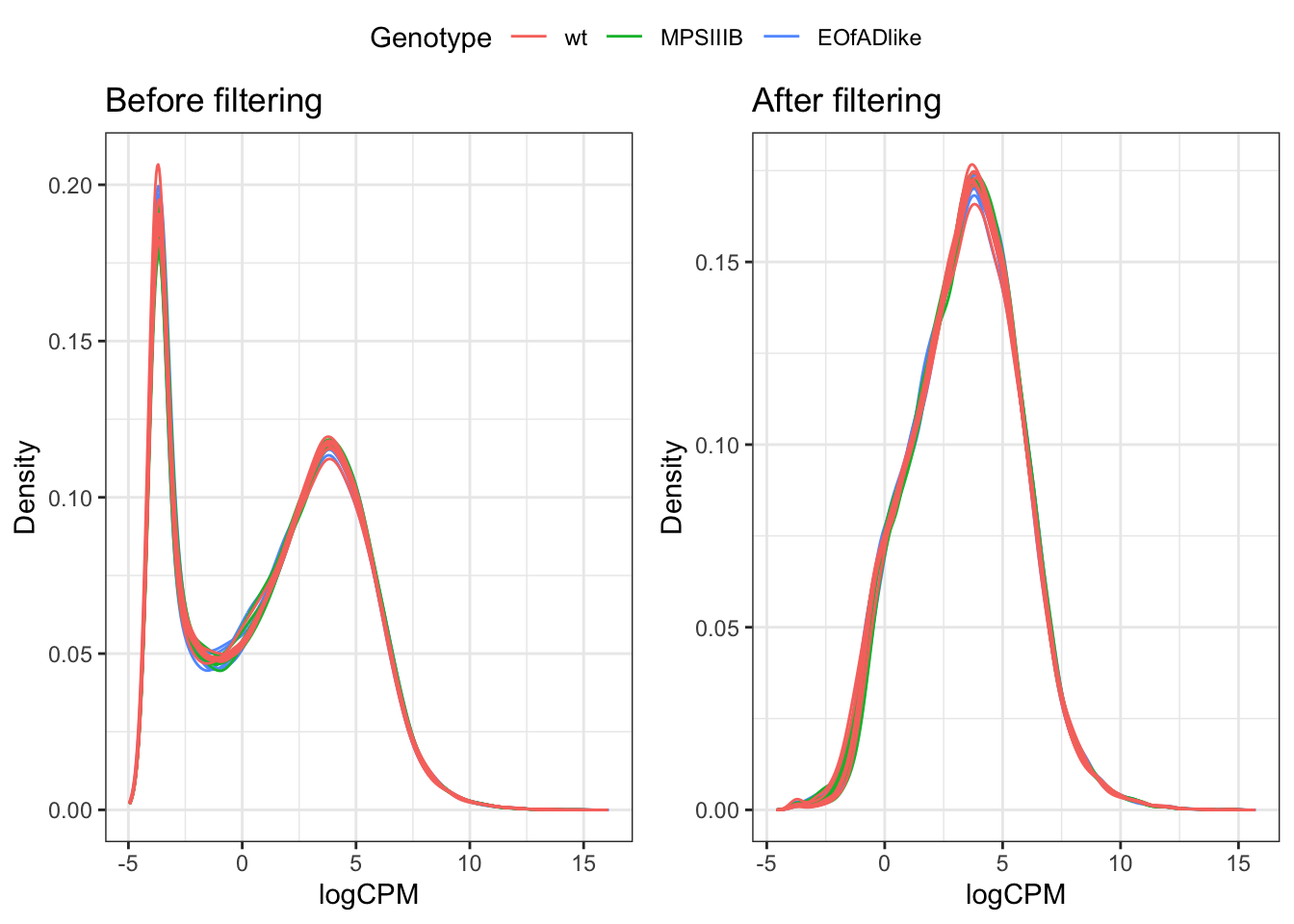

Version	Author	Date
0072e1a	Karissa Barthelson	2024-11-01

# make the DGE object, which contains information of genes, samples and metadata. 
x <- featureCounts %>% 
  as.matrix() %>% 
  .[rowSums(cpm(.) >= 0.5) >= 8,] %>% # filter out genes lowly expressed. 
  DGEList(
    samples = tibble(sample = colnames(.)) %>%
      left_join(meta),
    genes = grGenes[rownames(.)] %>%
      as.data.frame() %>%
      dplyr::select(
        chromosome = seqnames, start, end, 
        gene_id, gene_name, gene_biotype, description, entrezid
      ) %>% 
      left_join(gcGene) %>% 
      as_tibble()
  ) %>%
  calcNormFactors() # TMM normalisation - a standard method of normalisation in RNAseq data.

PCA

I first want to explore the overall similarity between samples by principal component analysis (PCA). PCA is a dimensionality reduction technique used to simplify complex datasets while retaining most of the important information. It works by transforming the original data into a new set of uncorrelated variables called principal components, which are linear combinations of the original variables. These components are ordered by the amount of variance they explain in the data, with the first principal component capturing the most variance. PCA is commonly used for visualization and to identify patterns or relationships in high-dimensional data. In the PCAs below, no distinct clusters of samples are observed by genotype.

x$counts %>% 
  cpm(log=TRUE) %>%  # convert counts to logCPM - standard measure of RNAseq data
  t() %>% # data meeds to be transposed for PCA (i.e. samples as rows, genes as columns)
  prcomp() %>% # perform PCA
  autoplot( # ggfortify package allows automatic plotting of prcomp outout 
    data = tibble(
      sample = rownames(.$x)
    ) %>% 
      left_join(x$samples),
    colour = "Genotype", 
    size = 6
  ) +
  theme(aspect.ratio = 1) +
  scale_color_discrete_qualitative(palette = "Dark 3") # change the colours.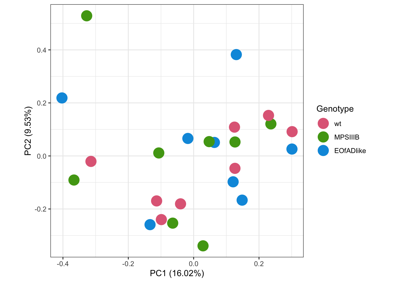

Version	Author	Date
0072e1a	Karissa Barthelson	2024-11-01

#  ggsave("output/plots/PCAblue.png", width = 10, height = 10, units = "cm", dpi = 300, scale = 1.25)

Also wanted to see if the RNA quality (i.e. the RIN) shows any patterns in the data, ubt

x$counts %>% 
  cpm(log=TRUE) %>% 
  t() %>% 
  prcomp() %>% 
  autoplot(data = tibble(sample = rownames(.$x)) %>%
      left_join(x$samples),
    colour = "RIN", 
    size = 6
  ) +
  theme_bw() + 
  theme(aspect.ratio = 1) +
  labs(colour = "RIN") +
  scale_color_viridis_c(end = 0.9)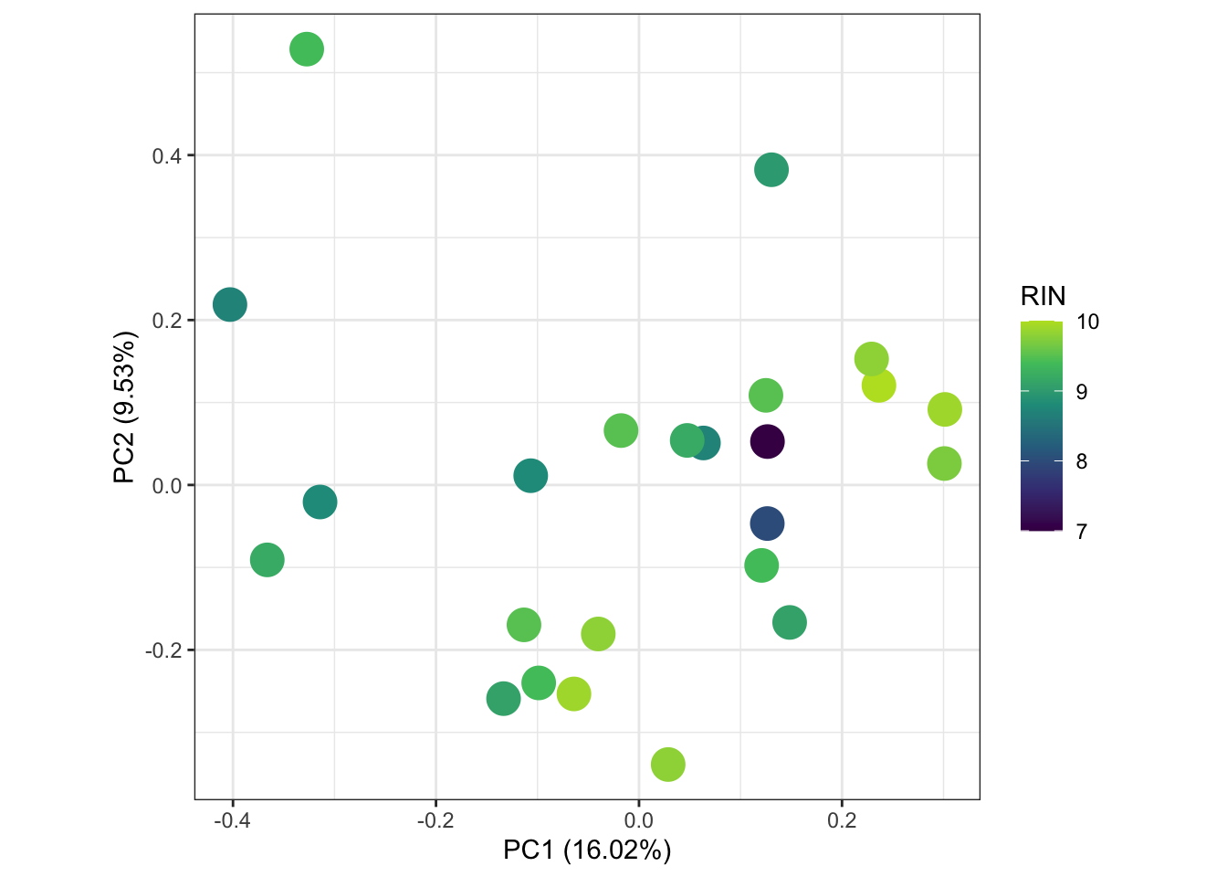

Version	Author	Date
0072e1a	Karissa Barthelson	2024-11-01

Check genotypes

The alignments (.bam files) were manually inspected using GViz to look at the sequence of the reads aligning to each of the mutation sites. Since this requires the HPC to be mounted to my computer, I have performed this seperately in the checkGenotypes.rmd file. All fish carry the genotypes indicated from the PCR genotyping.

%GC and Length check

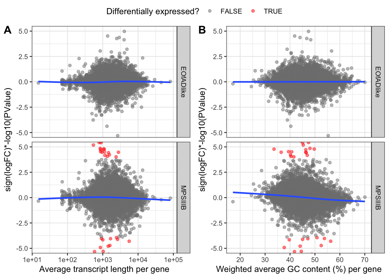
GC bias and length bias are common technical artifacts in RNA-seq data. GC bias occurs when sequences with higher or lower GC content are preferentially captured or sequenced, leading to inaccuracies in transcript quantification. Similarly, length bias arises because longer transcripts are more likely to generate more reads, making their expression levels appear higher. These biases can distort downstream analyses. Here, I will perform an initial DE gene analysis using edgeR and see if there are any trends for differential expression of genes due to their %GC or transcript length.

# create a design matrix, with an intercept as rhe WT genotype and each mut as the coefs. 
# a nice explanation of design matrices from the amazing bioinformaticians at WEHI can be found here: 
# https://bioconductor.org/packages/release/workflows/vignettes/RNAseq123/inst/doc/designmatrices.html
design <- model.matrix(~Genotype, data = x$samples) %>% 
  set_colnames(gsub(colnames(.), pattern = "Genotype", replacement = ""))

# fit generalised linear modes (negative binomial districbution) 
fit_1 <- x %>% 
  estimateDisp(design) %>% # estimate dispersions. 
  glmFit(design) # fit model

# Call the toptable (i.e. DE genes spreadsheet)
# this recursively performs the DE gene testing for each coefficient
toptable_1 <- design %>% colnames() %>% .[2:3] %>% 
  sapply(function(x){
    glmLRT(fit_1, coef = x) %>% # perform liklihood ratio tests
      topTags(n = Inf) %>% # create the spreadsheet 
      .[["table"]] %>%
      as_tibble() %>%
      arrange(PValue) %>%
       mutate(
        coef = x,
        DE = FDR < 0.05
      ) %>% 
      dplyr::select(
        # setup how i like it. 
        gene_name, logFC, logCPM, PValue, FDR, DE, everything()  
      )
      
  }, simplify = FALSE)

These plots are zoomed in between -10 and 10 on the y-axisfor vis purposes. the blue lines of best fit are a bit wonky, meaning there are some biases here for %GC and Length. Therefore, conditional quantile normailsation is required.

ggarrange(
toptable_1 %>% 
  bind_rows() %>% 
  mutate(rankstat = sign(logFC)*-log10(PValue)) %>% 
  ggplot(aes(x = length, y = rankstat)) +
  geom_point(
    aes(colour = DE),
    alpha = 0.5
  ) +
  geom_smooth(se = FALSE, method = "gam") +
  facet_grid(rows = vars(coef)) +
  theme_bw() +
  theme(legend.position = "none") +
  scale_color_manual(values = c("grey50", "red")) +
  scale_x_log10()+
  labs(x = "Average transcript length per gene",
       colour = "Differentially expressed?",
       y = "sign(logFC)*-log10(PValue)") +
  coord_cartesian(ylim = c(-5, 5)),

toptable_1 %>% 
  bind_rows() %>% 
  mutate(rankstat = sign(logFC)*-log10(PValue)) %>% 
  ggplot(aes(x = gc_content, y = rankstat)) +
  geom_point(
    aes(colour = DE),
    alpha = 0.5
  ) +
  geom_smooth(se = FALSE, method = "gam") +
  facet_grid(rows = vars(coef)) +
  theme_bw() +
  theme(legend.position = "none") +
  scale_color_manual(values = c("grey50", "red")) +
  coord_cartesian(ylim = c(-5,5)) + 
  labs(x = "Weighted average GC content (%) per gene", 
       colour = "Differentially expressed?", 
       y = "sign(logFC)*-log10(PValue)"),
common.legend = TRUE, 
labels = "AUTO"
)

Version	Author	Date
0072e1a	Karissa Barthelson	2024-11-01

CQN

Here, I will apply the cqn correction to adjust for the observed bias for %GC and length.

cqn <-   
x %>% 
  with(
    cqn(
      counts = counts,
      x = genes$gc_content,
      lengths = genes$length,
      sizeFactors = samples$lib.size
    )
  )
logCPM <- cqn$y + cqn$offset

par(mfrow = c(1, 2))
cqnplot(cqn, n = 1, xlab = "GC Content")
cqnplot(cqn, n = 2, xlab = "Length")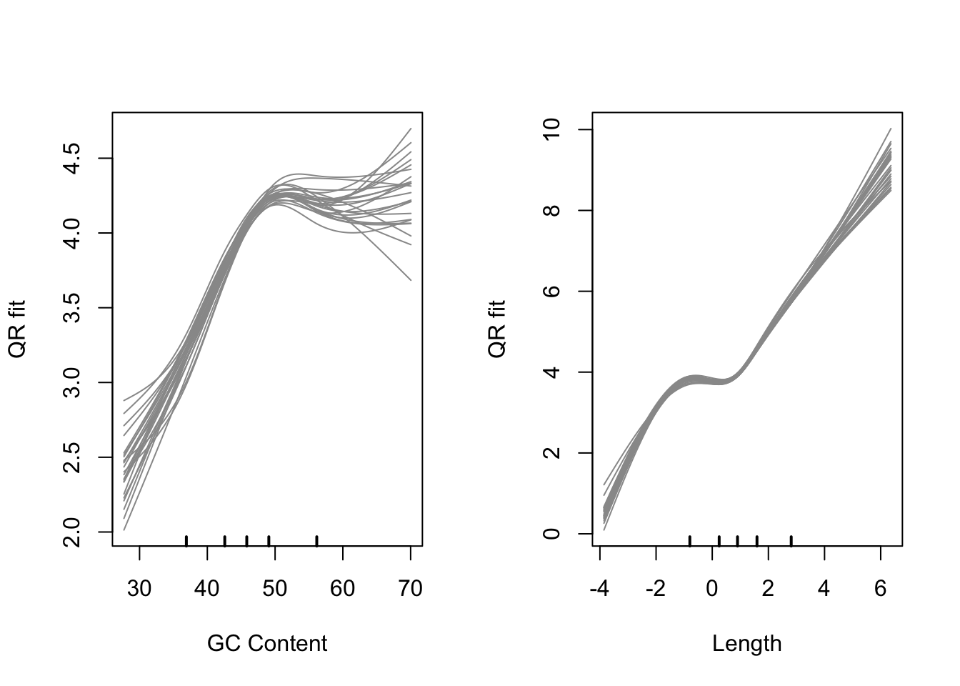

Model fits for GC content and gene length under the CQN model. Variability is clearly visible at either end

Version	Author	Date
0072e1a	Karissa Barthelson	2024-11-01

par(mfrow = c(1, 1))

PCA after cqn

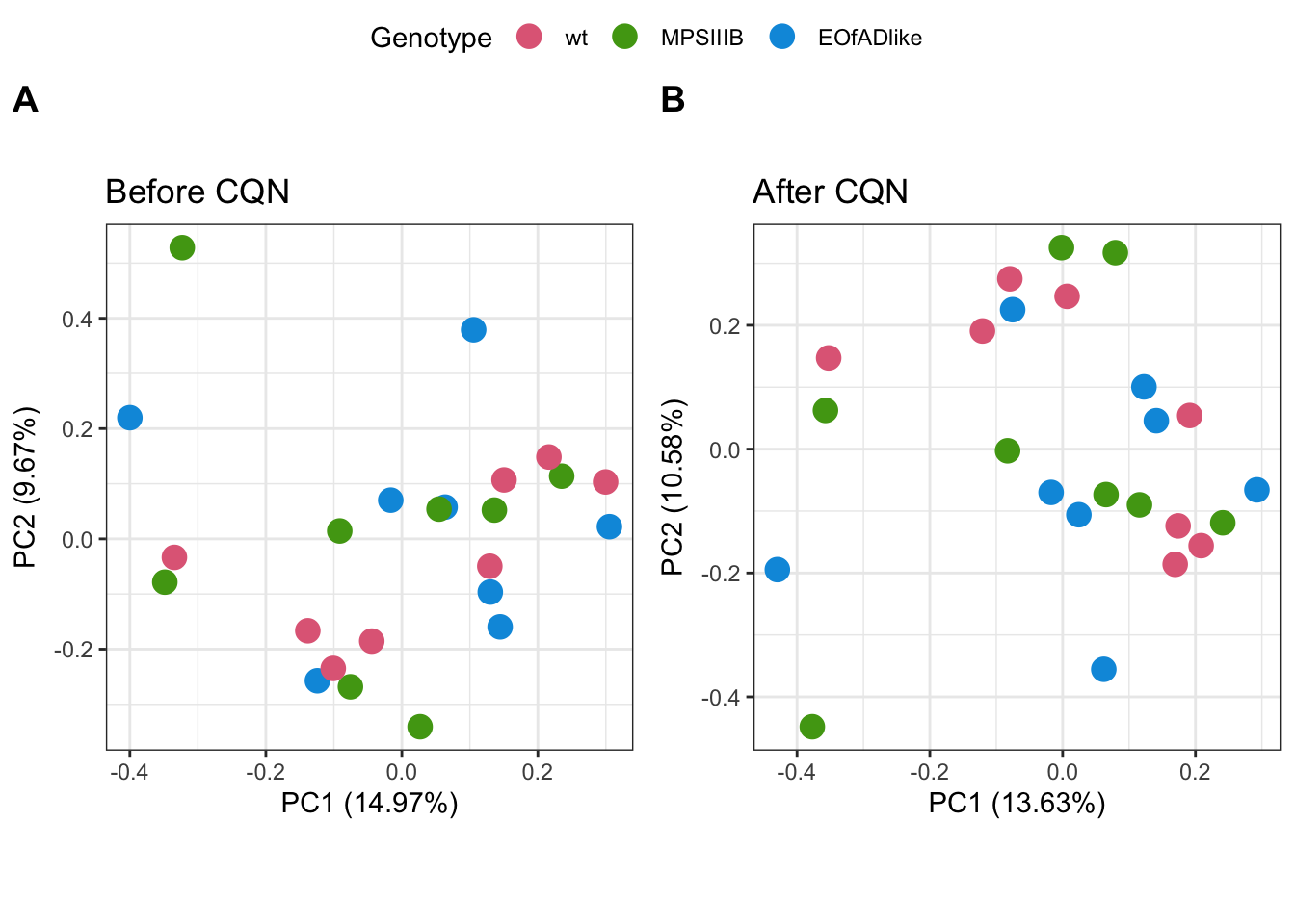
PCA analysis was repeated. No significant improvement of clustering of samples by genotype is observed

ggarrange(
  cpm(x, log = T) %>%
    t() %>%
    prcomp() %>% 
    autoplot(data = tibble(sample = rownames(.$x)) %>%
               left_join(x$samples),
             colour = "Genotype", 
             
             size = 4
    ) +
    scale_color_discrete_qualitative(palette = "Dark 3") +
    theme(aspect.ratio = 1) +
    ggtitle("Before CQN"),
  
  logCPM %>% 
    t() %>% 
    prcomp() %>%
    autoplot(data = tibble(sample = rownames(.$x)) %>%
               left_join(x$samples),
             colour = "Genotype", 
             size = 4
    ) +
    scale_color_discrete_qualitative(palette = "Dark 3") +
    theme(aspect.ratio = 1) +
    ggtitle("After CQN"),
  common.legend = T, 
  labels = "AUTO"
)

Version	Author	Date
0072e1a	Karissa Barthelson	2024-11-01

DE with cqn

CQN generates an “offset” which is included in the generalised linear models fitted in edgeR. Here, I repeat the edgeR model fitting & DE analysis including this offset.

# Add the offset to the dge object 
x$offset <- cqn$glm.offset

# fit the glm
fit_cqn <- x %>% 
  estimateDisp(design) %>% 
  glmFit(design)

# call the toptables. 
toptables_cqn <- design %>% colnames() %>% .[2:3] %>% 
  sapply(function(x){
    glmLRT(fit_cqn, coef = x) %>%
      topTags(n = Inf) %>%
      .[["table"]] %>%
      as_tibble() %>%
      arrange(PValue) %>%
       mutate(
        coef = x,
        DE = FDR < 0.05
      ) %>% 
      dplyr::select(
        gene_name, logFC, logCPM, PValue, FDR, DE, everything()  
      )
      
  }, simplify = FALSE)

Visualisation of DE genes

Volcano plot

toptables_cqn %>%
  bind_rows() %>% 
  ggplot(aes(y = -log10(PValue), x = logFC, colour = DE)) +
  geom_point(
    alpha = 0.5, size = 1.25
  ) +
  facet_wrap(~coef) +
  # geom_label_repel(
  #   aes(label = gene_name),
  #   data = .  %>% dplyr::filter(FDR < 0.05),
  #   show.legend = FALSE
  #   ) +
  coord_cartesian(xlim = c(-2.5,2.5), 
                  ylim = c(0, 20) )+
  theme(legend.position = "none") +
  scale_color_manual(values = c("grey50", "red"))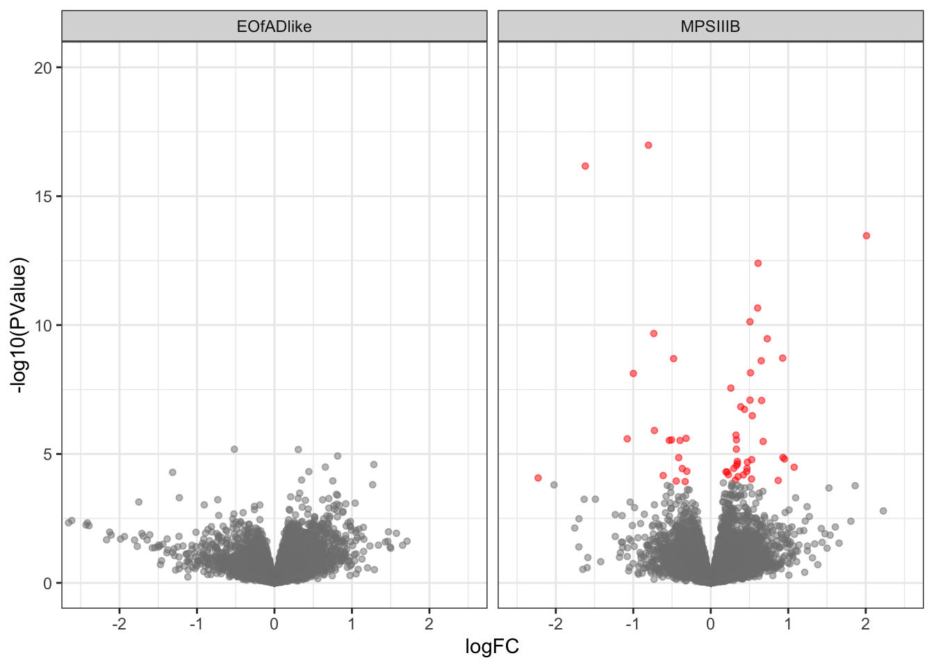

Version	Author	Date
0072e1a	Karissa Barthelson	2024-11-01

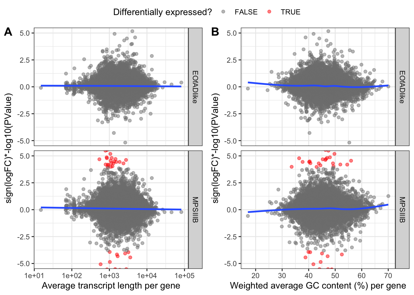
rech-check the %GC & length bias

Doesnt look like CQN did a whole lot here. But will still include it.

ggarrange(
toptables_cqn %>% 
  bind_rows() %>% 
  mutate(rankstat = sign(logFC)*-log10(PValue)) %>% 
  ggplot(aes(x = length, y = rankstat)) +
  geom_point(
    aes(colour = DE),
    alpha = 0.5
  ) +
  geom_smooth(se = FALSE, method = "gam") +
  facet_grid(rows = vars(coef)) +
  theme_bw() +
  theme(legend.position = "none") +
  scale_color_manual(values = c("grey50", "red")) +
  scale_x_log10()+
  labs(x = "Average transcript length per gene",
       colour = "Differentially expressed?",
       y = "sign(logFC)*-log10(PValue)") +
  coord_cartesian(ylim = c(-5, 5)),

toptables_cqn %>% 
  bind_rows() %>% 
  mutate(rankstat = sign(logFC)*-log10(PValue)) %>% 
  ggplot(aes(x = gc_content, y = rankstat)) +
  geom_point(
    aes(colour = DE),
    alpha = 0.5
  ) +
  geom_smooth(se = FALSE, method = "gam") +
  facet_grid(rows = vars(coef)) +
  theme_bw() +
  theme(legend.position = "none") +
  scale_color_manual(values = c("grey50", "red")) +
  coord_cartesian(ylim = c(-5,5)) + 
  labs(x = "Weighted average GC content (%) per gene", 
       colour = "Differentially expressed?", 
       y = "sign(logFC)*-log10(PValue)"),
common.legend = TRUE, 
labels = "AUTO"
)

Gene set enrichment analysis

I now will perform some gene set enrichment analyses to assess the bioloigcal meaning of the DE genes. I will use gene sets obtained from MSigDB (Molecular Signatures Database). This is a curated collection of gene sets used for functional enrichment and pathway analysis. It is widely utilized in genomics research to interpret high-throughput expression data by linking genes or transcripts to known biological pathways, cellular processes, or molecular functions.

Gene sets

The gene sets I will test will be the following:

KEGG: Canonical Pathways gene sets derived from the KEGG pathway database. Note that I should use the KEGG medicus gene sets in the future.

# d/l the KEGG gene sets and setup in list format by gene ids. 
KEGG <- msigdbr(
  species = "Danio rerio",
  category = "C2", subcategory = "CP:KEGG"
) %>% 
  left_join(x$genes, by = c("gene_symbol" = "gene_name")) %>% # add the ens gene ids
  dplyr::filter(gene_id %in% rownames(x)) %>% # only retain genes detected in this RNAseq exp. 
  distinct(gs_name, gene_id, .keep_all = TRUE) %>% # keep unique 
  split(f = .$gs_name) %>%
  lapply(extract2, "gene_id")

Gene ontologies: GO is a collaborative effort to develop and use ontologies to support biologically meaningful annotation of genes and their products. A GO annotation consists of a GO term associated with a specific reference that describes the work or analysis upon which the association between a specific GO term and gene product is based. Each annotation also includes an evidence code to indicate how the annotation to a particular term is supported (http://geneontology.org/page/guide-go-evidence-codes). Gene sets in this subcollection are prefixed with “GOBP” (Biological Process), “GOMF” (Molecular Function), or “GOCC” (Cellular Component) to indicate their source ontology.

# GO Terms
# get the GO summaries that Stevie generated way back
# this is to help reduce redundant GO terms. 
goSummaries <- url("https://uofabioinformaticshub.github.io/summaries2GO/data/goSummaries.RDS") %>%
  readRDS() %>%
  mutate(
    Term = Term(id),
    gs_name = Term %>% str_to_upper() %>% str_replace_all("[ -]", "_"),
    gs_name = paste0("GO_", gs_name)
    )

# define this as the min path
minPath <- 3

GO <-
  msigdbr("Danio rerio", category = "C5") %>%
  dplyr::filter(grepl(gs_name, pattern = "^GO")) %>%
  left_join(x$genes, by = c("gene_symbol" = "gene_name")) %>%
  dplyr::filter(gene_id %in% rownames(x)) %>%
  # omit these prefixes - im not interested in them for this analysis. 
  mutate(gs_name = str_replace(gs_name, pattern = "GOBP_", replacement = "GO_")) %>% 
  mutate(gs_name = str_replace(gs_name, pattern = "GOMF_", replacement = "GO_")) %>%
  mutate(gs_name = str_replace(gs_name, pattern = "GOCC_", replacement = "GO_")) %>%
  left_join(goSummaries) %>%
  dplyr::filter(shortest_path >= minPath) %>%
  distinct(gs_name, gene_id, .keep_all = TRUE) %>%
  split(f = .$gs_name) %>%
  lapply(extract2, "gene_id")

# calculate the sizes of the GO terms.  
sizes_GO <- GO %>%
  lapply(length) %>%
  unlist %>%
  as.data.frame() %>%
  set_colnames( "n_genes") %>%
  rownames_to_column("gs")

# retain gene sets with at least 3 genes in it
GO <- GO[sizes_GO %>% dplyr::filter(n_genes > 3) %>% .$gs]

Iron-responsive element gene sets Dr. Nhi Hin developed gene sets which are responsive to intracellular iron levels. Changes to the expression of these genes can represent changes to intracellular iron levels. For more details - see her amazing [paper](https://pubmed.ncbi.nlm.nih.gov/34719489/.

I went to her GitHub repo and downloaded the rds file for the zebrafish IRE genes.

ireGenes <- readRDS("data/gene_sets/zebrafishireGenes.rds") %>% 
  unlist() %>% 
  as.data.frame() %>% 
  rownames_to_column("ire") %>% 
  as_tibble() %>% 
  mutate(ire = str_extract(ire, pattern = "ire[:digit:]_[:alpha:]+")) %>% 
  set_colnames(c("ire", "gene_id")) %>% 
  dplyr::filter(gene_id %in% rownames(x)) %>% 
  split(f = .$ire) %>% 
  lapply(magrittr::extract2,"gene_id")

Chromosome location gene sets

We often see DE genes arising from the same chromosome of the mutation when comparing mutant genotypes. This can indicate DE genes not related to the true biology of the mutation we are studying, rather it can represent other variants on the mutant chromosome which result in different gene expression values. See Baer et al. 2024 for a nice explanation of this.

chr <- x$genes %>% 
  dplyr::select(gene_id, chromosome) %>% 
  split(f = .$chromosome) %>%
  lapply(extract2, "gene_id") %>% 
  .[c("MT", seq(1:25))] # omit the ALT chromosmes and scaffolds

Cell type markers

Cell type marker gene sets are collections of genes that are specifically or highly expressed in particular cell types, serving as molecular signatures to identify those cells. We are analysiing bulk larval tissue, and so if there is a cell type missing (e.g. neurons) we would see downregulation of neuronal genes. This is an important interpretation of changes to gene expression - is it functional? or is it a cell type proportion change?

These gene sets come from Farnsworth et al.. Its a 5dpf scRNAseq dataset as I couldnt find a 7 dpf gene set in the literature.

# Cell type markers for zerbafish 
cell_type_markers <- read_excel("data/gene_sets/1-s2.0-S0012160619304919-mmc7.xlsx") %>% 
  dplyr::filter(grepl(`Day of Origin`, pattern = 5 )) %>%  # restrict to only 5dpf
  dplyr::select(Tissue, 9:24) %>% 
  split(f = .$Tissue) %>% 
  lapply(function(y) {
    y %>% 
      dplyr::select(-Tissue) %>% 
      gather %>% 
      dplyr::select(value) %>% 
      set_colnames("gene_name") %>% 
      left_join(x$genes) %>% 
      na.omit %>% 
      .$gene_id
  }) 

# get length of gene sets
sizes <- cell_type_markers %>% 
  lapply(length) %>% 
  unlist %>% 
  as.data.frame() %>% 
  set_colnames( "n_genes") %>% 
  rownames_to_column("gs")

# retain gene sets with at least 5 genes in it
cell_type_markers <- cell_type_markers[sizes %>% dplyr::filter(n_genes > 5) %>% .$gs]

Testing for over-representation of GO terms in the DE genes using GOSEQ

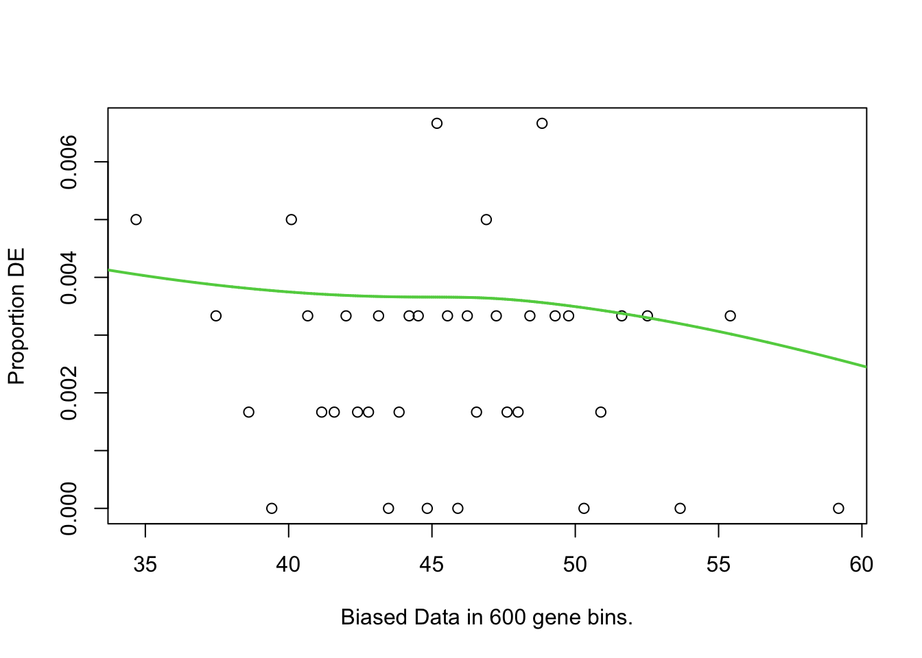
First, I will test for over-representation of GO terms within the DE genes. I will do this using goseq as it allows you to include a co-variate which is nice. Since there seems to still be a little bit of bias remaining for %GC content even after cqn, this is what I will specify as the covariate.

There were no DEGs in the EOfAD like mutatns, so no GO testing will be performed for this comparison.

The top 10 GO terms over-represented in the DEGs in MPS-IIIB are plotted below.

pwf <- toptables_cqn$MPSIIIB %>%
      with(
        nullp(
          DEgenes = structure(DE, names = gene_id), 
          bias.data = gc_content
        )
      )

goseq_mpsiiib <- goseq(pwf, gene2cat = GO) %>% 
  as_tibble() %>% 
  dplyr::filter(numDEInCat > 0) %>% 
  mutate(FDR = p.adjust(over_represented_pvalue, method = "fdr")) %>% 
  dplyr::select(-under_represented_pvalue) 

goseq_mpsiiib %>%
  dplyr::slice(1:10) %>%
  mutate(propDE = numDEInCat/numInCat) %>%
  ggplot(aes(x = -log10(over_represented_pvalue), y = reorder(category, -over_represented_pvalue))) +
  geom_col(aes(fill = propDE, alpha = FDR < 0.05)) +
  scale_fill_viridis_c() +
  scale_alpha_manual(values = c(0.4, 1)) +
  labs(y = "GO Term",
       fill = "Proportion of \nDE genes in \nGO term")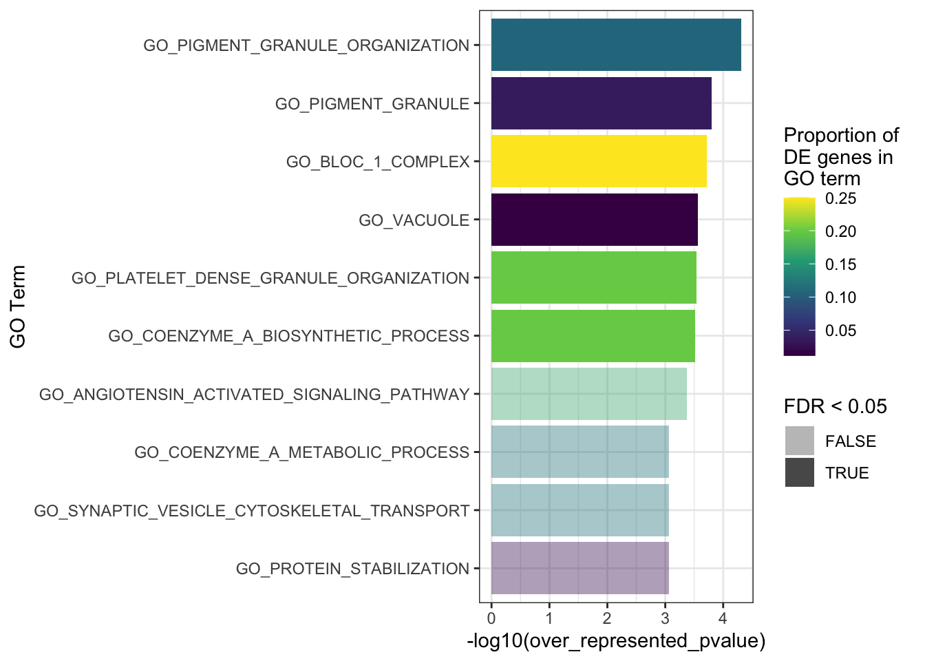

Ranked-list approach to gene set testing with fry

Overrepresenation analysis using goseq relies on a hard threshold for gene to be called DE. This can lose information as there are genes which are almost DE (i.e. FDRp = 0.06), but are not interpreted in this way.

Another method to test for enrichment of gene sets is to use ROAST. Roast uses a rotation-based approach to generate a null distribution of gene set enrichment scores by randomly permuting the samples or the gene labels in the data. Roast then calculates a gene set enrichment score for each gene set in the data, based on the correlation between the gene expression values and the sample labels. The gene set enrichment scores are compared to the null distribution to calculate the statistical significance of the enrichment. In this way, it does not requre a list of DEGs as input.

Here, I will perform the fast approx of ROAST: fry, from the limma package on the KEGG gene sets. The top 10 gene sets in each mutant zebrafish are shown below.

KEGG

fryKEGG <- 
  design %>% colnames() %>% .[2:3] %>% 
  sapply(function(y) {
   logCPM %>% 
      fry(
        index = KEGG,
        design = design, 
        contrast = y, 
        sort = "mixed"
      ) %>% 
      rownames_to_column("pathway") %>% 
      as_tibble() %>% 
      mutate(coef = y)
  }, simplify = FALSE)

fryKEGG$MPSIIIB %>% 
  dplyr::slice(1:10) %>% 
  mutate(pathway = str_remove(pathway, pattern = "KEGG_")) %>% 
  ggplot(aes(x = -log10(PValue.Mixed), y = reorder(pathway, -PValue.Mixed))) +
  geom_col(aes(fill = FDR.Mixed < 0.05)) +
  scale_fill_manual(values = c("grey50", 'red')) +
  theme_pubr() +
  labs(fill = "FDR < 0.05", 
       x = "-log10(PValue)", 
       y = "", 
       title = "MPS-IIIB")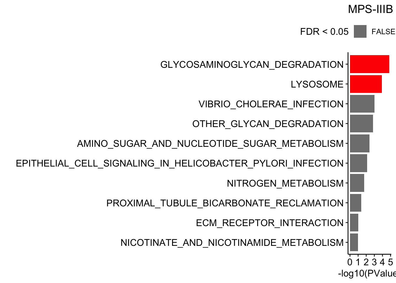

  #theme(text = element_text(size = 40)) 
  # ggsave("output/plots/geneSetsInMPS-IIIB.png", width = 10, height = 7, 
  #        units = "cm", dpi = 300, scale= 5)
  

fryKEGG$EOfADlike %>% 
  dplyr::slice(1:10) %>% 
  mutate(pathway = str_remove(pathway, pattern = "KEGG_")) %>% 
  ggplot(aes(x = -log10(PValue.Mixed), y = reorder(pathway, -PValue.Mixed))) +
  geom_col(aes(fill = FDR.Mixed < 0.05)) +
  scale_fill_manual(values = c("grey50", 'red')) +
  theme_pubr() +
  labs(fill = "FDR < 0.05", 
       x = "-log10(PValue)", 
       y = "", 
       title = "EOfAD")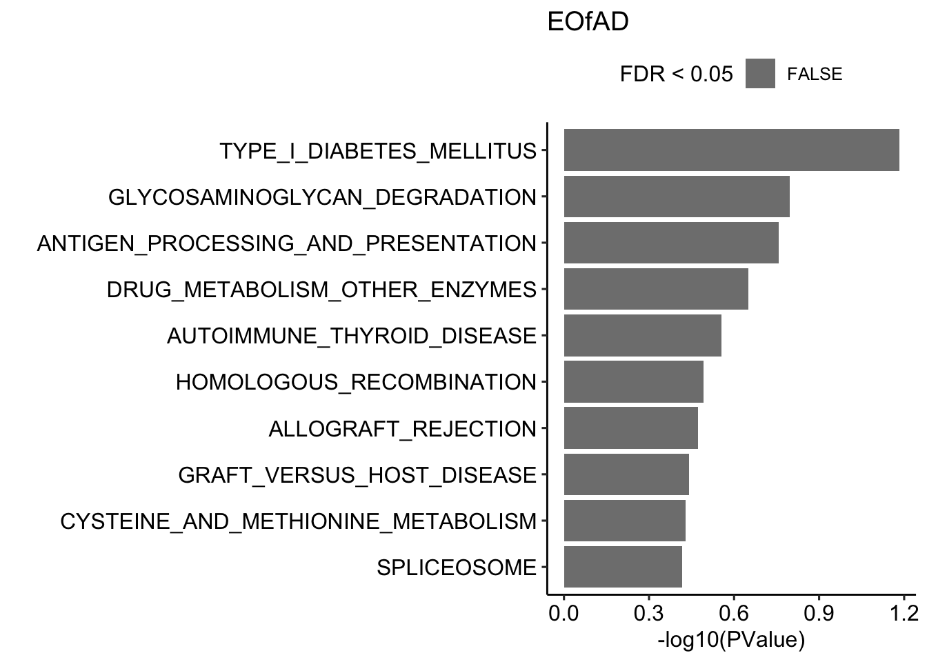

IRE

Statistical significance in these iron-responsive element gene sets can indicate iron dyshomoestasis.

fryIRE <- design %>% colnames() %>% .[2:3] %>% 
  sapply(function(y) {
    cpm(x$counts, log = TRUE) %>% 
      fry(
        index = ireGenes,
        design = design, 
        contrast = y, 
        sort = "directional"
      ) %>% 
      rownames_to_column("pathway") %>% 
      as_tibble() %>% 
      mutate(coef = y)
  }, simplify = FALSE)

fryIRE %>% 
  bind_rows() %>% 
  dplyr::select(pathway, coef, pvalue = PValue.Mixed, FDR = FDR.Mixed) %>% 
  ggplot(aes(y = pathway, x = -log10(pvalue))) + 
  geom_col(aes(fill = coef), 
           position = "dodge") +
  geom_vline(xintercept = -log10(0.05)) +
  scale_fill_viridis_d(end = 0.75) +
  theme_pubr()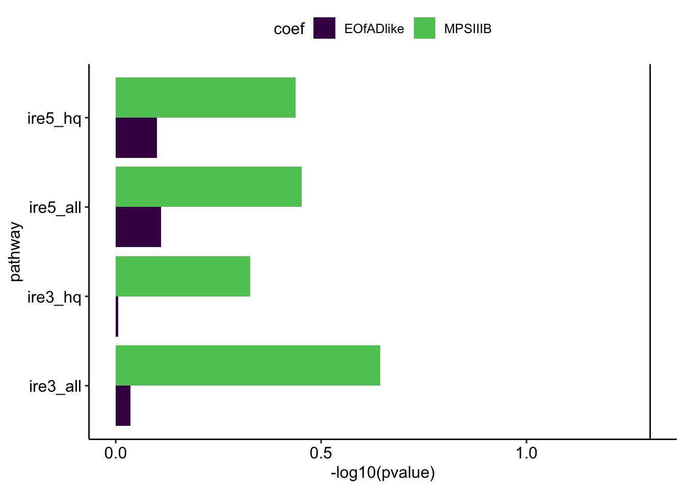

Version	Author	Date
0072e1a	Karissa Barthelson	2024-11-01

  #ggsave("output/plots/ire.png", width = 10, height = 10, units = "cm", dpi = 300)

Cell type prop check

Since this experiment was performed on whole larvae, we need to have a look at whether changes to cell type proportions could explain cause some artefactual changes to gene expression. We have done this previously by assessing the expression of marker genes of specific cell types. So this is what I will do here. I have taken the lists of genes frmo day 5 only from the zebrafish single cell atlas (Farnsworth et al. 2020) which contain at least 10 genes. This leaves 24 gene sets (cell types) to test.

fry.cell <- design %>% colnames() %>% .[2:3] %>% 
  sapply(function(y) {
    cpm(x$counts, log = TRUE) %>% 
      fry(
        index = cell_type_markers,
        design = design, 
        contrast = y, 
        sort = "directional"
      ) %>% 
      rownames_to_column("pathway") %>% 
      as_tibble() %>% 
      mutate(coef = y) %>% 
      dplyr::select(1:5)
  }, simplify = FALSE)

Chromosome gene sets

Are there DEGs on the mutant chromosomes?

design %>% colnames() %>% .[2:3] %>% 
  sapply(function(y) {
    cpm(x$counts, log = TRUE) %>% 
      fry(
        index = c(chr),
        design = design, 
        contrast = y, 
        sort = "mixed"
      ) %>% 
      rownames_to_column("pathway") %>% 
      as_tibble() %>% 
      mutate(coef = y)
  }, simplify = FALSE)

$MPSIIIB
# A tibble: 26 × 8
   pathway NGenes Direction PValue   FDR PValue.Mixed     FDR.Mixed coef   
   <chr>    <int> <chr>      <dbl> <dbl>        <dbl>         <dbl> <chr>  
 1 24         615 Up        0.258  0.280     2.44e-10 0.00000000634 MPSIIIB
 2 25         665 Up        0.0147 0.179     3.25e- 3 0.0423        MPSIIIB
 3 8          939 Up        0.115  0.179     1.40e- 1 0.508         MPSIIIB
 4 5         1219 Up        0.0729 0.179     1.75e- 1 0.508         MPSIIIB
 5 17         819 Up        0.115  0.179     1.81e- 1 0.508         MPSIIIB
 6 14         763 Up        0.122  0.179     1.94e- 1 0.508         MPSIIIB
 7 3         1176 Up        0.166  0.188     2.12e- 1 0.508         MPSIIIB
 8 15         825 Up        0.101  0.179     2.36e- 1 0.508         MPSIIIB
 9 12         770 Up        0.160  0.188     2.36e- 1 0.508         MPSIIIB
10 11         734 Up        0.138  0.179     2.41e- 1 0.508         MPSIIIB
# ℹ 16 more rows

$EOfADlike
# A tibble: 26 × 8
   pathway NGenes Direction PValue   FDR PValue.Mixed FDR.Mixed coef     
   <chr>    <int> <chr>      <dbl> <dbl>        <dbl>     <dbl> <chr>    
 1 17         819 Up         0.781 0.846        0.226     0.986 EOfADlike
 2 18         697 Up         0.557 0.752        0.473     0.986 EOfADlike
 3 9          817 Up         0.474 0.752        0.513     0.986 EOfADlike
 4 25         665 Up         0.237 0.752        0.548     0.986 EOfADlike
 5 23         834 Up         0.613 0.752        0.643     0.986 EOfADlike
 6 2         1055 Up         0.577 0.752        0.661     0.986 EOfADlike
 7 3         1176 Up         0.631 0.752        0.696     0.986 EOfADlike
 8 4         1084 Down       0.986 0.990        0.799     0.986 EOfADlike
 9 8          939 Up         0.689 0.779        0.874     0.986 EOfADlike
10 14         763 Up         0.636 0.752        0.874     0.986 EOfADlike
# ℹ 16 more rows

Harmonic mean p

Since I’m not detecting any significant gene sets in the EOfAD-like mutants, I need to try another method. I will use the harmonic mean p val method which combines indivisual p vals from 3 gene set enrichmen analysis methods: fry, camera and gsea.

# Make a custom function for calculating the HMP.  
runHMP = function(gene.set.obj, 
                  design,
                  logCPM.df, 
                  toptable) {
fry <- 
  design %>% colnames() %>% .[2:3] %>% 
  sapply(function(y) {
  logCPM.df %>% 
      fry(
        index = gene.set.obj,
        design = design, 
        contrast = y, 
        sort = "mixed"
      ) %>% 
      rownames_to_column("pathway") %>% 
      as_tibble() %>% 
      mutate(coef = y)
  }, simplify = FALSE)

camera <- 
  design %>% colnames() %>% .[2:3] %>% 
  sapply(function(y) {
    logCPM.df %>% 
      camera(
        index = gene.set.obj,
        design = design, 
        contrast = y
      ) %>% 
      rownames_to_column("pathway") %>% 
      as_tibble() %>% 
      mutate(coef = y)
  }, simplify = FALSE)

ranks <- 
   sapply(toptable, function(y) {
     y %>% 
       mutate(rankstat = sign(logFC) * log10(1/PValue)) %>% 
       arrange(rankstat) %>% 
       dplyr::select(c("gene_id", "rankstat")) %>% #only want the Pvalue with sign
       with(structure(rankstat, names = gene_id)) %>% 
       rev() # reverse so the start of the list is upregulated genes
   }, simplify = FALSE)

# Run fgsea

# set a seed for a reproducible result
set.seed(33)
fgsea <- ranks %>%
  sapply(function(x){
    fgseaMultilevel(stats = x, pathways = gene.set.obj) %>%
      as_tibble() %>%
      dplyr::rename(FDR = padj) %>%
      mutate(padj = p.adjust(pval, "bonferroni")) %>%
      dplyr::select(pathway, pval, FDR, padj, everything()) %>%
      arrange(pval) %>%
      mutate(sig = padj < 0.05)
  }, simplify = F)

fgsea$MPSIIIB %<>% 
  mutate(coef = "MPSIIIB")
fgsea$EOfADlike %<>% 
  mutate(coef = "EOfADlike")

hmp <- fry %>% 
  bind_rows() %>% 
  dplyr::select(pathway, PValue.Mixed, coef) %>% 
  dplyr::rename(fry_p = PValue.Mixed) %>% 
  left_join(camera %>% 
              bind_rows() %>% 
              dplyr::select(pathway, PValue, coef), 
            by = c("pathway", "coef")) %>% 
  dplyr::rename(camera_p = PValue) %>% 
  left_join(fgsea %>% 
              bind_rows() %>% 
              dplyr::select(pathway, pval, coef), 
            by = c("pathway", "coef")) %>% 
  dplyr::rename(fgsea_p = pval) %>% 
  bind_rows() %>% 
  nest(p = one_of(c("fry_p", "camera_p", "fgsea_p"))) %>% 
 mutate(harmonic_p = vapply(p, function(x){
        x <- unlist(x)
        x <- x[!is.na(x)]
        p.hmp(x, L = 4)
      }, numeric(1))
 ) %>% 
  unnest() %>% 
  mutate(harmonic_p_FDR = p.adjust(harmonic_p, "fdr"),
         sig = harmonic_p_FDR < 0.05) %>% 
  arrange(harmonic_p) 

return(list(
  hmp = hmp, 
  fgsea = fgsea
))

}

KEGG

HMP_kegg <- runHMP(gene.set.obj = KEGG, 
                   design = design, 
                   logCPM.df = logCPM, 
                   toptable = toptables_cqn)

sigpaths <- HMP_kegg$hmp %>% 
  dplyr::filter(harmonic_p_FDR < 0.05) %>% 
  .$pathway

HMP_kegg$hmp %>% 
  dplyr::filter(pathway %in% sigpaths) %>% 
  ggplot(aes(x = coef, y = reorder(pathway, -harmonic_p))) + 
  geom_tile(aes(fill = -log10(harmonic_p), 
                alpha = sig)) +
  geom_label(aes(label = signif(harmonic_p_FDR, digits = 2)), 
             fill = NA) +
  scale_fill_viridis_c()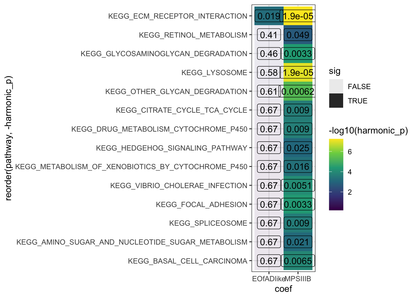

Version	Author	Date
0072e1a	Karissa Barthelson	2024-11-01

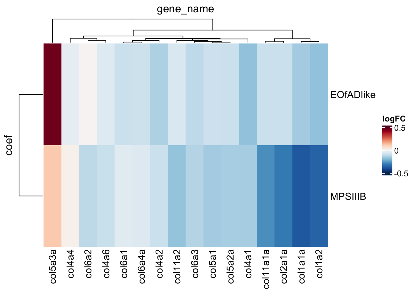
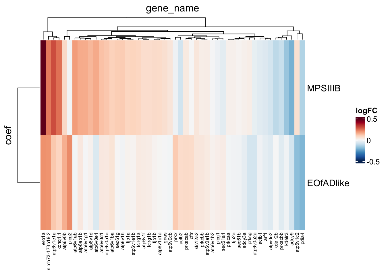
ECM

Plot the ECM logFC values t look at directionality

toptables_cqn %>% 
  bind_rows() %>% 
  dplyr::filter(
    gene_id %in% KEGG$KEGG_ECM_RECEPTOR_INTERACTION
    ) %>% 
  dplyr::filter(
    grepl(description, pattern = "collag")
  ) %>% 
  dplyr::distinct(
    gene_name, coef, .keep_all = TRUE
  ) %>% 
  heatmap(
    .row = coef,
    .col = gene_name, 
    .value = logFC, 
    
    palette_value = circlize::colorRamp2(
            seq(-0.5, 0.5, length.out = 11), 
            rev(RColorBrewer::brewer.pal(11, "RdBu"))
    )
  )

Version	Author	Date
0072e1a	Karissa Barthelson	2024-11-01

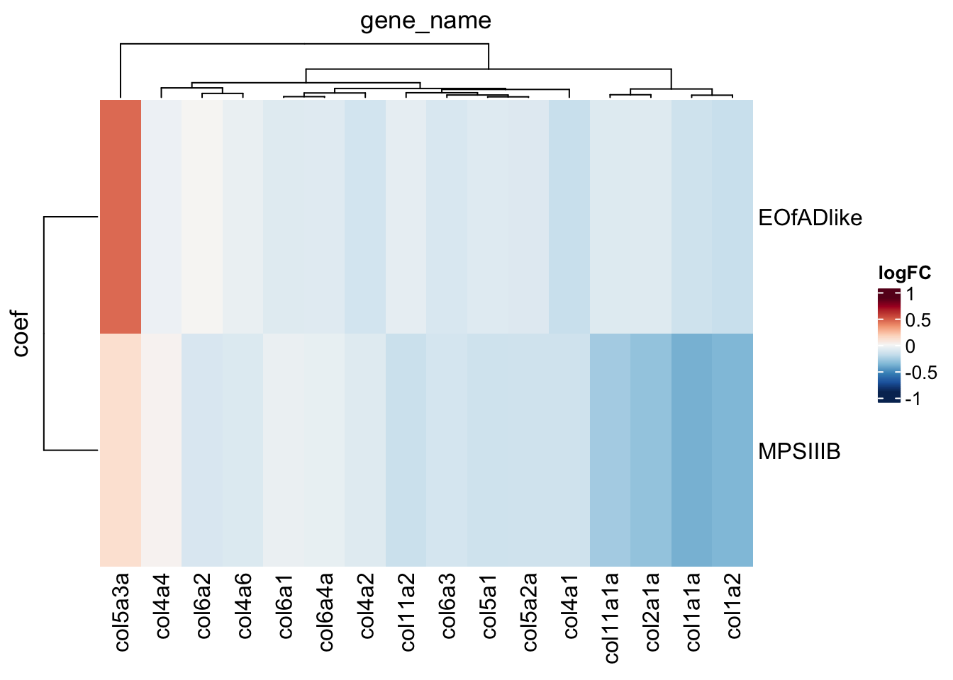
# save as an svg for the paper

# svg("output/plots4pub3/ECM_collagen_larvae_hm.svg", 
#    width = 10, height = 3)

# look at the collagen genes specifically

toptables_cqn %>% 
  bind_rows() %>% 
  dplyr::filter(
    gene_id %in% KEGG$KEGG_ECM_RECEPTOR_INTERACTION
    ) %>% 
  dplyr::filter(
    grepl(description, pattern = "collag")
  ) %>% 
  dplyr::distinct(
    gene_name, coef, .keep_all = TRUE
  ) %>% 
  heatmap(
    .row = coef,
    .col = gene_name, 
    .value = logFC, 
    
    palette_value = circlize::colorRamp2(
            seq(-0.9, 0.9, length.out = 11), 
            rev(RColorBrewer::brewer.pal(11, "RdBu"))), 
  )

#  dev.off()

vibrio cholarae infection gene set

Kim was interested in this gene set - so want to see what genes are driving its statistical significnace .

toptables_cqn %>% 
  bind_rows() %>% 
  dplyr::filter(
    gene_id %in% KEGG$KEGG_VIBRIO_CHOLERAE_INFECTION
    ) %>% 
  dplyr::distinct(
    gene_name, coef, .keep_all = TRUE
  ) %>% 
  heatmap(
    .row = coef,
    .col = gene_name, 
    .value = logFC, 
      
    
    palette_value = circlize::colorRamp2(
            seq(-0.5, 0.5, length.out = 11), 
            rev(RColorBrewer::brewer.pal(11, "RdBu"))
    )
  )

Version	Author	Date
0072e1a	Karissa Barthelson	2024-11-01

IRE

No staistical significance in the IRE genes

HMP_ire <- runHMP(gene.set.obj = ireGenes, 
                   design = design, 
                   logCPM.df = logCPM, 
                   toptable = toptables_cqn)


HMP_ire$hmp %>% 
  ggplot(aes(x = coef, y = reorder(pathway, -harmonic_p))) + 
  geom_tile(aes(fill = -log10(harmonic_p), 
                alpha = sig)) +
  geom_label(aes(label = signif(harmonic_p_FDR, digits = 2)), 
             fill = NA) +
  scale_fill_viridis_c()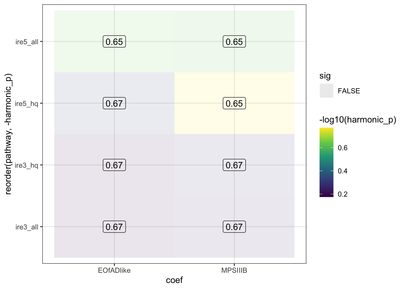

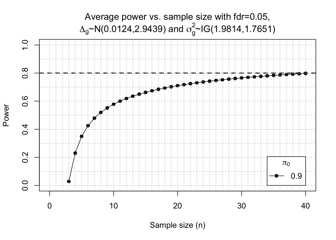
Post-hoc power calculation

Since we were detetcting much DE genes in the EOfAD-like mutants, i wanted to check what level of statistcial power we achived here. This can be done using the package ssizeRNA

# set a seed for a reroducilble result. 
set.seed(2016)

# this was largely followed from the vigentte of the package. 
mu <- x$counts %>%
  as.data.frame() %>%
  .[grepl(colnames(x$counts), pattern = "wt")] %>%
  rowMeans()

disp <-  x %>% estimateDisp() %>% . $tagwise.dispersion

fc <- function(y){exp(rnorm(y, log(1), 0.5*log(2)))}

power <- ssizeRNA_vary(nGenes = dim(x)[1], # Num detectable genes
              pi0 = 0.9, # Proportion of non-DE genes
              m = 30, # pseudo sample size
              mu = mu, # Average read count for each gene in control group. Calculated from this current dataset)
              disp = disp, # Dispersion parameter for each gene
              fc = fc, # Fold change per gene
              fdr = 0.05, # FDR level to control
              #power = 0.7, # power level
              maxN = 40,
              replace = T
                )

# plot the power myself/ 
power$power %>% 
  set_colnames(c("n", "power")) %>% 
  ggplot(aes(x = n, y = power)) +
  geom_point() +
  geom_line() +
  coord_cartesian(xlim = c(0,30)) +
  geom_hline(yintercept = 0.7, linetype = 2, colour = "red") +
  geom_hline(yintercept = 0.51, linetype = 2, colour = "blue")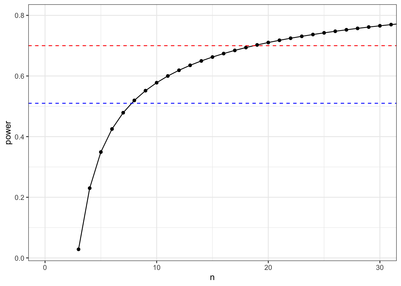

  #ggsave("output/plots/posthocPowerLarvae.png", width = 10, height = 5, units = "cm", 
   #      dpi = 200, scale = 1.5)

Note for Anqi - you can stop here. the rest of this doc is quite specific to my paper.

Compare with Dong et al. data

Yang had previously analysed the EOfADlike mutation in pools of larvae. Here, I want to see how similar my results are.

Obtained his github repo from here, which has the data https://github.com/yangdongau/20190717_Lardelli_RNASeq_Larvae

Comparing his fc vales im not really seeing much. I wil re-process his data to do HMP analyses on it.

x.Dong <- read_rds("data/DongEtAlData/dgeList.rds")

x.Dong$samples %<>% 
  mutate(Genotype = case_when(
    Genotype == "Q96K97del/+" ~ "EOfADlike", 
    Genotype == "WT" ~ "wt"
  ) %>% 
    factor(levels = c("wt", "EOfADlike")))

larvaeGenos <- x.Dong$samples %>% 
  dplyr::select(Genotype) %>% 
  mutate(exp = "pools") %>% 
  bind_rows(x$samples %>% dplyr::select(Genotype) %>% mutate(exp = "individual")) %>% 
  rownames_to_column("sample")

# PCA
cpm(x, log = T) %>% 
  as.data.frame() %>% 
  rownames_to_column("gene_id") %>% 
  left_join(x.Dong$counts %>% cpm(log=T) %>% as.data.frame %>% rownames_to_column("gene_id")) %>% 
  column_to_rownames("gene_id") %>% 
  dplyr::select(!starts_with("MPS")) %>% 
  na.omit %>% 
  t %>% 
  prcomp() %>% 
  autoplot(data = tibble(sample = rownames(.$x)) %>%
             left_join(larvaeGenos),
           colour = "Genotype", 
           size = 4
  ) +
  geom_mark_ellipse(aes(labels = exp)) +
  scale_color_discrete_qualitative(palette = "Dark 3") +
  theme(aspect.ratio = 1)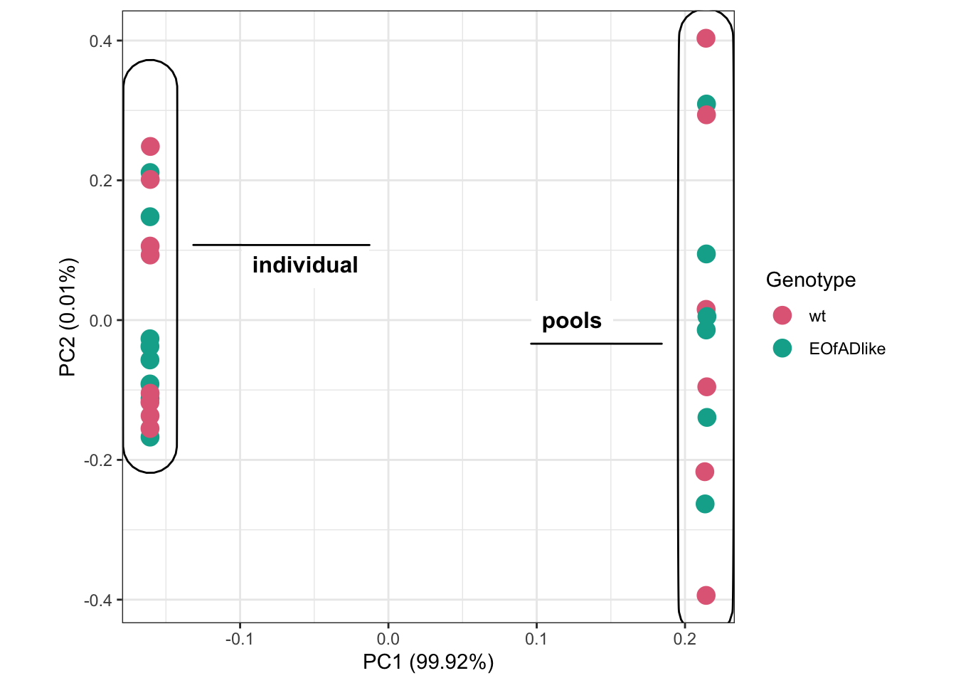

# suss out ECM
toptable_dongetal <- 
  read_csv("data/DongEtAlData/topTable.csv") %>% 
  dplyr::rename( gene_id = ensembl_gene_id, 
                 gene_name = external_gene_name)

toptable_dongetal %>% 
  dplyr::filter(gene_id %in% KEGG$KEGG_ECM_RECEPTOR_INTERACTION) %>% 
  dplyr::select(gene_name, logFC.pools = logFC) %>% 
  left_join(toptables_cqn$EOfADlike %>% dplyr::select(gene_name, logFC.individuals = logFC)) %>% 
  dplyr::distinct(gene_name, .keep_all = T) %>% 
  column_to_rownames("gene_name") %>% 
  pheatmap(color = colorRampPalette(rev(brewer.pal(n = 5,
                                               name = "RdBu")))(200), 
           breaks = seq(-0.6, 0.6, by = 0.6*2/200), 
           main ="KEGG_ECM_RECEPTOR_INTERACTION")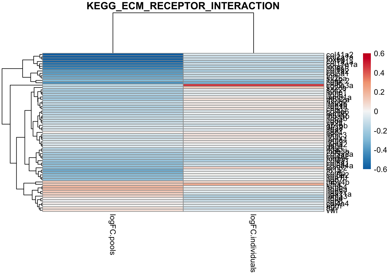

toptable_dongetal %>% 
  dplyr::filter(gene_id %in% KEGG$KEGG_ECM_RECEPTOR_INTERACTION) %>% 
  dplyr::select(gene_name, logFC.pools = logFC) %>% 
    left_join(toptables_cqn$EOfADlike %>% dplyr::select(gene_name, logFC.individuals = logFC)) %>% 
  dplyr::distinct(gene_name, .keep_all = T) %>% 
  column_to_rownames("gene_name") %>% 
  ggscatter(x = "logFC.individuals", y = "logFC.pools",
   color = "black", shape = 21, size = 3, # Points color, shape and size
   add = "reg.line",  # Add regressin line
   add.params = list(color = "blue", fill = "lightgray"), # Customize reg. line
   conf.int = TRUE, # Add confidence interval
   cor.coef = TRUE, # Add correlation coefficient. see ?stat_cor
   #cor.coeff.args = list(method = "pearson", label.x = 3, label.sep = "\n")
   ) +
  geom_abline(slope = 1) +
  labs(title = "Pearson corr of genes in KEGG_ECM_RECEPTOR_INTERACTION")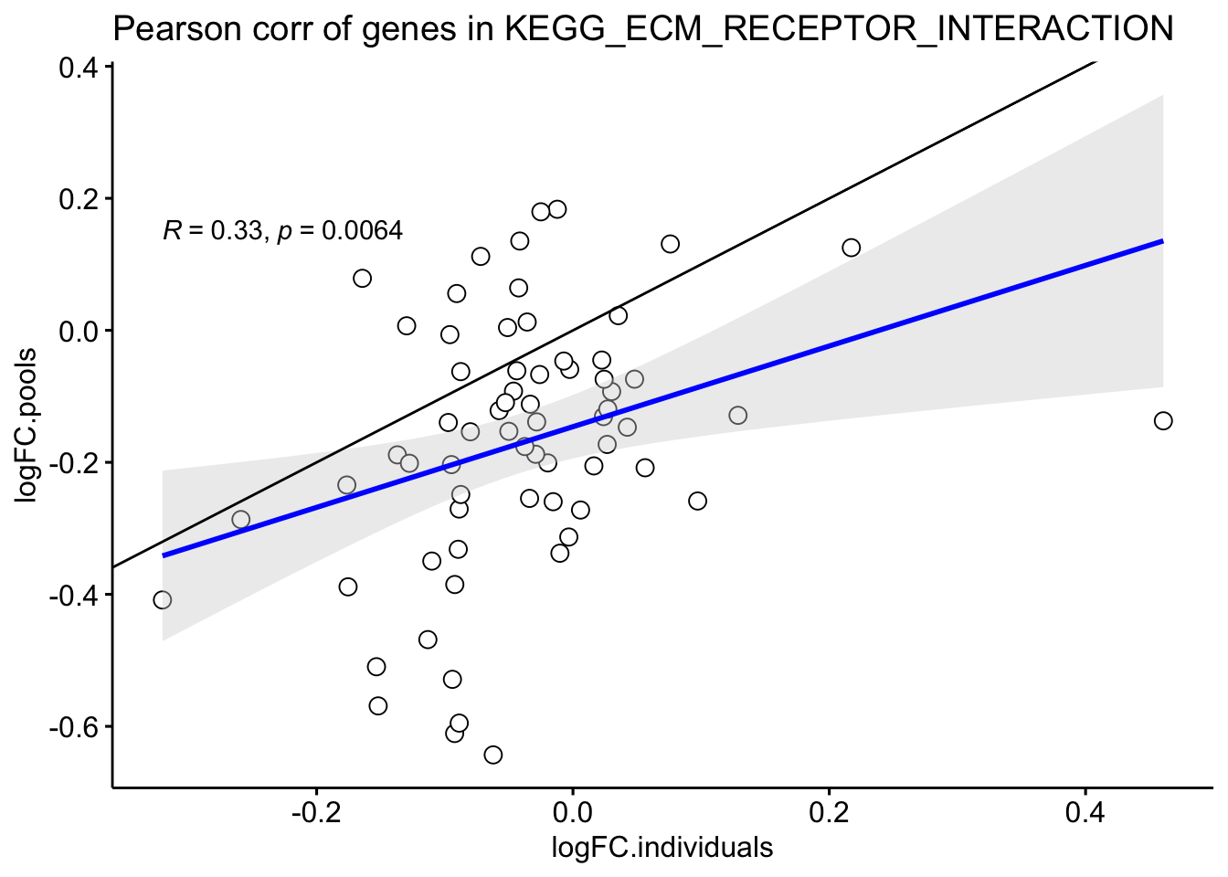

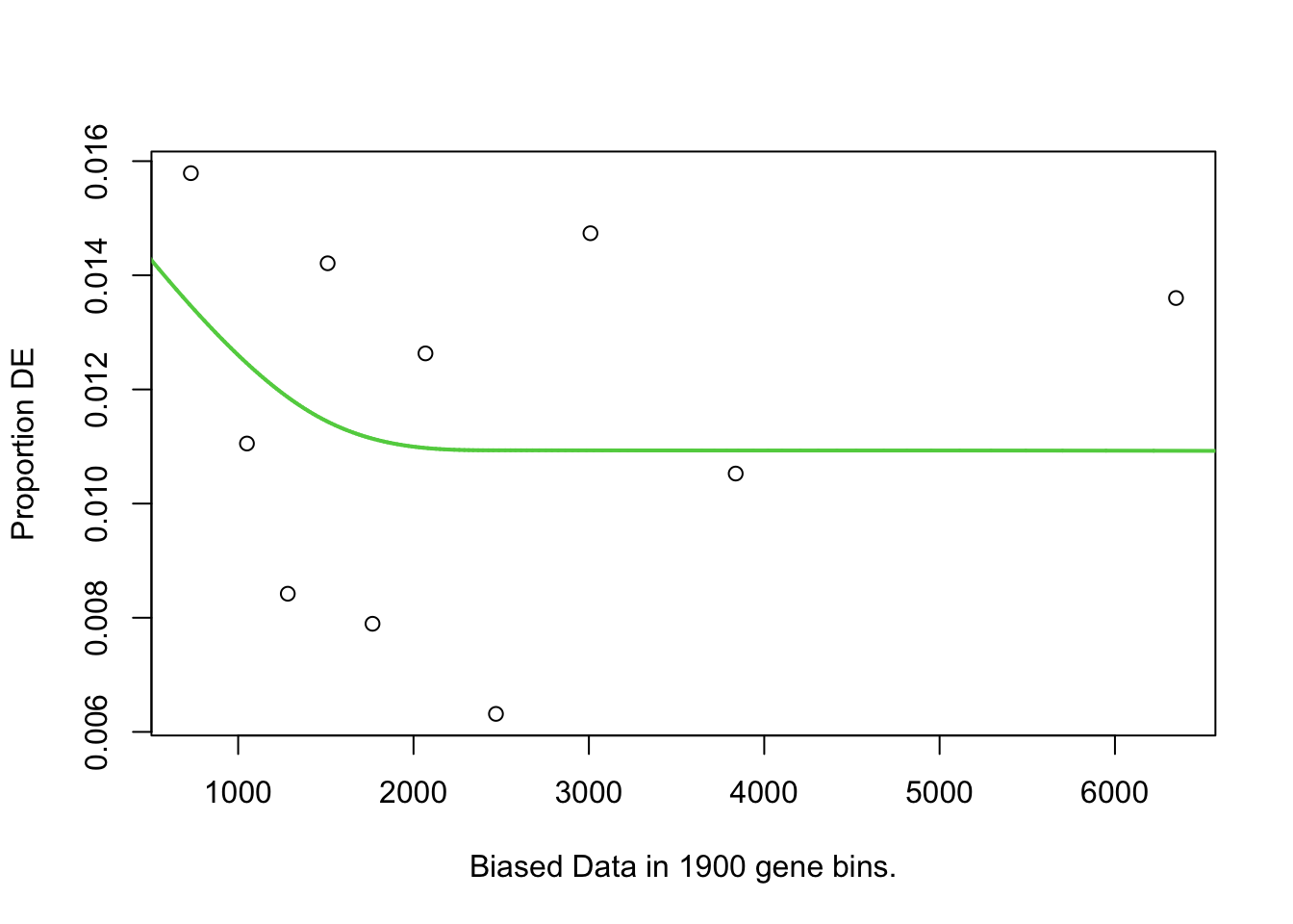
pwf.dong <- toptable_dongetal %>%
      with(
        nullp(
          DEgenes = structure(DE, names = gene_id), 
          bias.data = aveLength 
        )
      )

goseq_dong <- goseq(pwf.dong, gene2cat = GO) %>% 
  as_tibble() %>% 
  #dplyr::filter(numDEInCat > 0) %>% 
  mutate(FDR = p.adjust(over_represented_pvalue, method = "fdr")) %>% 
  dplyr::select(-under_represented_pvalue) 

goseq_dong %>% dplyr::filter(category == "GO_PROTON_TRANSPORTING_V_TYPE_ATPASE_COMPLEX")

# A tibble: 1 × 5
  category                      over_represented_pva…¹ numDEInCat numInCat   FDR
  <chr>                                          <dbl>      <int>    <int> <dbl>
1 GO_PROTON_TRANSPORTING_V_TYP…                      1          0       25     1
# ℹ abbreviated name: ¹over_represented_pvalue

goseq_mpsiiib %>% 
  dplyr::slice(1:10) %>% 
  mutate(propDE = numDEInCat/numInCat) %>% 
  ggplot(aes(x = -log10(over_represented_pvalue), y = reorder(category, -over_represented_pvalue))) +
  geom_col(aes(fill = propDE, alpha = FDR < 0.05)) +
  scale_fill_viridis_c() +
  scale_alpha_manual(values = c(0.4, 1)) +
  labs(y = "GO Term", 
       fill = "Proportion of \nDE genes in \nGO term")

HMP with dong et al.

design.dong <- model.matrix(~Genotype + W_1, x.Dong$samples) %>% 
  set_colnames(str_replace(colnames(.), pattern = "Genotype.+", "EOfAD-like"))

fry <- 
  cpm(x.Dong, log = T) %>% 
      fry(
        index = KEGG,
        design = design.dong, 
        contrast = "EOfAD-like", 
        sort = "mixed"
      ) %>% 
      rownames_to_column("pathway") %>% 
      as_tibble() %>% 
      mutate(coef = "EOfAD-like", 
             sig = FDR.Mixed < 0.05)

camera <- 
  cpm(x.Dong, log = T) %>% 
  camera(
    index = KEGG,
    design = design.dong, 
    contrast = "EOfAD-like"
  ) %>% 
      rownames_to_column("pathway") %>% 
      as_tibble() %>% 
      mutate(coef = "EOfAD-like")

ranks <- 
  toptable_dongetal %>% 
  mutate(rankstat = sign(logFC) * log10(1/PValue)) %>% 
  arrange(rankstat) %>% 
  dplyr::select(c("gene_id", "rankstat")) %>% #only want the Pvalue with sign
  with(structure(rankstat, names = gene_id)) %>% 
  rev() # reverse so the start of the list is upregulated genes

# Run fgsea

# set a seed for a reproducible result
set.seed(33)
fgsea <- ranks %>%
  fgseaMultilevel(pathways = KEGG) %>%
  as_tibble() %>%
  dplyr::rename(FDR = padj) %>%
  mutate(padj = p.adjust(pval, "bonferroni")) %>%
  dplyr::select(pathway, pval, FDR, padj, everything()) %>%
  arrange(pval) %>%
  mutate(sig = padj < 0.05, 
         coef ="EOfAD-like")

hmp.dong <- fry %>% 
  dplyr::select(pathway, PValue.Mixed, coef) %>% 
  dplyr::rename(fry_p = PValue.Mixed) %>% 
  left_join(camera %>% 
              dplyr::select(pathway, PValue, coef), 
            by = c("pathway", "coef")) %>% 
  dplyr::rename(camera_p = PValue) %>% 
  left_join(fgsea %>% 
              bind_rows() %>% 
              dplyr::select(pathway, pval, coef), 
            by = c("pathway", "coef")) %>% 
  dplyr::rename(fgsea_p = pval) %>% 
  bind_rows() %>% 
  nest(p = one_of(c("fry_p", "camera_p", "fgsea_p"))) %>% 
 mutate(harmonic_p = vapply(p, function(x){
        x <- unlist(x)
        x <- x[!is.na(x)]
        p.hmp(x, L = 4)
      }, numeric(1))
 ) %>% 
  unnest() %>% 
  mutate(harmonic_p_FDR = p.adjust(harmonic_p, "fdr"),
         sig = harmonic_p_FDR < 0.05) %>% 
  arrange(harmonic_p) 

hmp.kegg.q96 <- hmp.dong %>% 
  mutate(exp = "pools") %>% 
  bind_rows(HMP_kegg$hmp %>% 
              mutate(exp = "individuals")) %>% 
  dplyr::filter(coef == "EOfADlike")

sig.q96 <- hmp.kegg.q96 %>% 
  dplyr::filter(sig == T) %>% 
  .$pathway %>% 
  unique

hmp.dong %>% 
  dplyr::filter(pathway %in% sig.q96) %>% 
  ggplot(aes(x = -log10(harmonic_p), y = reorder(pathway, -harmonic_p))) +
  geom_col(aes(fill = -log10(harmonic_p))) +
  scale_fill_viridis_c() +
  theme_classic()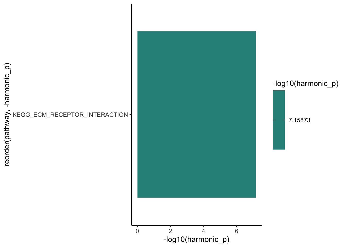

does Genotype drive the Dong ECM?

form <- ~ (1|Genotype) + (1|pair)
geneExpr <- 
  x.Dong$counts #%>% 
    # as.data.frame() %>% 
    # rownames_to_column("gene_id") %>% 
    # dplyr::filter(gene_id %in% KEGG$KEGG_ECM_RECEPTOR_INTERACTION) %>% 
    # column_to_rownames("gene_id")
#
n <- parallel::detectCores()/2 # experiment!
cl <- parallel::makeCluster(n)
doParallel::registerDoParallel(cl)

# this takes forever to run.
#varpar <- fitExtractVarPartModel(geneExpr, form, x.Dong$samples, 
#                                 BPPARAM=SnowParam(1)) # turn off parallel as my laptop sucks
#saveRDS(varpar, "data/dongvarpar.rds")                
varpar <- readRDS("data/dongvarpar.rds")

varpar %>% 
  .[KEGG$KEGG_ECM_RECEPTOR_INTERACTION,] %>% 
  rownames_to_column("gene_id") %>% 
  na.omit %>% 
  arrange(Genotype) %>% 
  gather(key = "var", value = "prop", c(Genotype, pair, Residuals)) %>% 
  ggplot(aes(x = var, y = prop)) +
  geom_violin() +
  geom_boxplot(width = 0.1)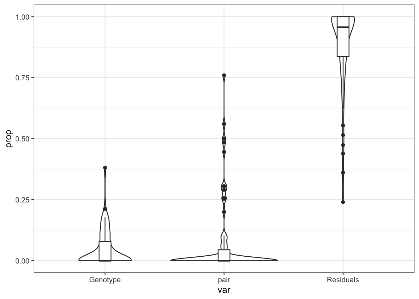

## power calc Dong # Post-hoc power calc

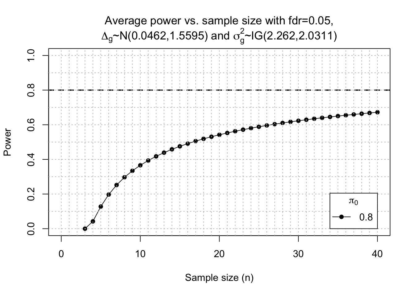
set.seed(2016)

mu2 <- 
  x.Dong$counts %>%
  as.data.frame() %>%
  .[,(x.Dong$samples %>% dplyr::filter(Genotype == "wt") %>% .$sample)] %>%
  rowMeans()

disp2 <-  x.Dong %>% estimateDisp() %>% . $tagwise.dispersion

fc <- function(y){exp(rnorm(y, log(1), 0.5*log(1.5)))}

power2 <- ssizeRNA_vary(nGenes = dim(x.Dong)[1], # Num detectable genes
              pi0 = 0.8, # Proportion of non-DE genes
              m = 30, # pseudo sample size
              mu = mu2, # Average read count for each gene in control group. Calculated from this current dataset)
              disp = disp2, # Dispersion parameter for each gene
              fc = fc, # Fold change per gene
              fdr = 0.05, # FDR level to control
              #power = 0.7, # power level
              maxN = 40,
              replace = T
                )

power2$power %>% 
  set_colnames(c("n", "power")) %>% 
  ggplot(aes(x = n, y = power)) +
  geom_point() +
  geom_line() +
  coord_cartesian(xlim = c(0,30)) +
  geom_vline(xintercept = 8)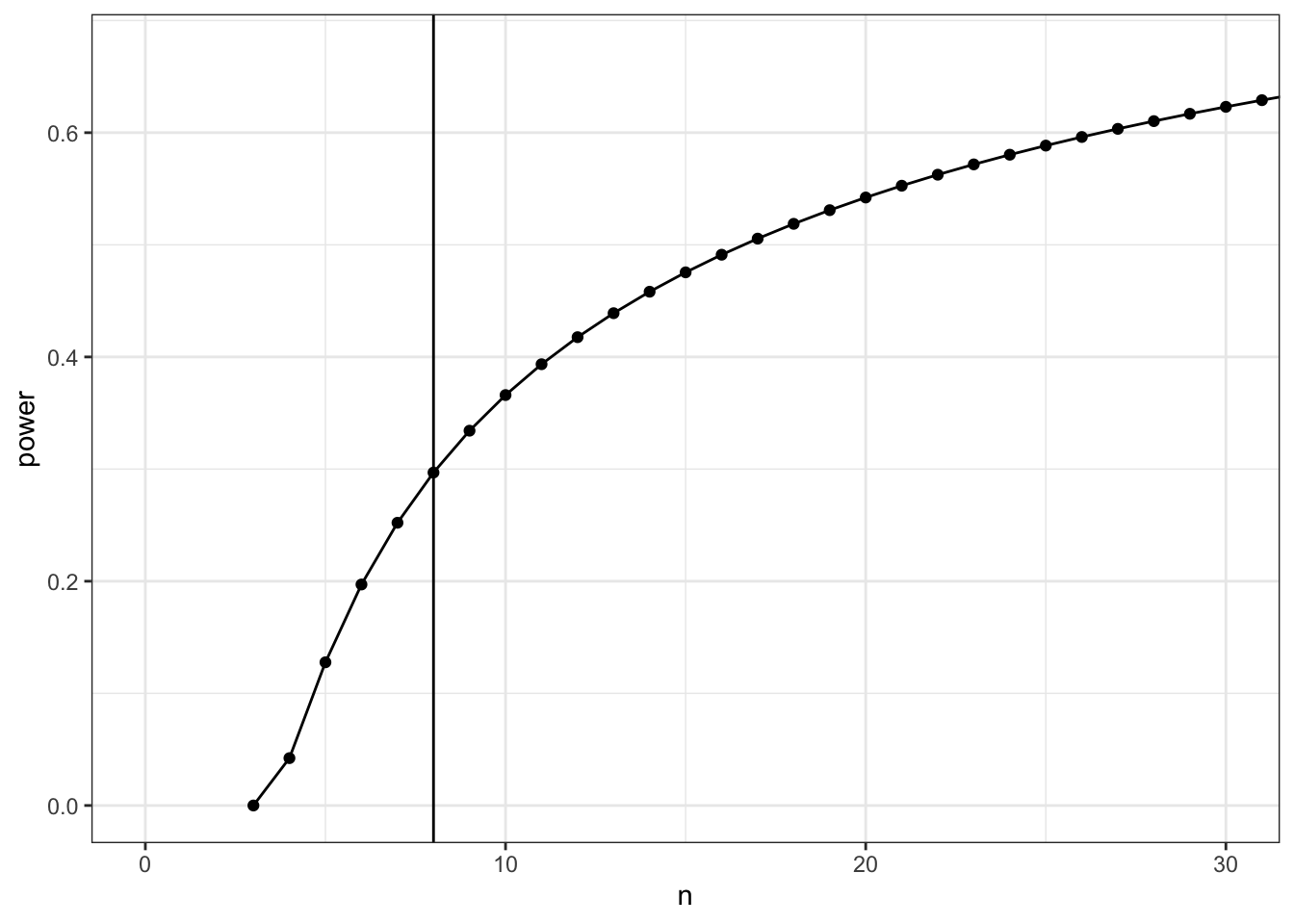

  geom_hline(yintercept = 0.51, linetype = 2, colour = "blue")

mapping: yintercept = ~yintercept 
geom_hline: na.rm = FALSE
stat_identity: na.rm = FALSE
position_identity

  # ggsave("output/plots/posthocPowerLarvae.png", width = 10, height = 5, units = "cm", 
  #        dpi = 200, scale = 1.5)

Data export

x %>% saveRDS("data/R_objects/larvae/dge.rds")
logCPM %>% saveRDS("data/R_objects/larvae/logcpm.rds")
toptables_cqn %>% saveRDS("data/R_objects/larvae/toptablescqn.rds")
HMP_kegg %>% saveRDS("data/R_objects/larvae/hmp_kegg.rds")
HMP_ire %>% saveRDS("data/R_objects/larvae/hmp_ire.rds")
fry.cell %>% saveRDS("data/R_objects/larvae/celltype_larvae.rds")

# 
# ire.output <- HMP_ire$hmp %>% 
#   left_join(HMP_ire$fgsea %>% 
#               bind_rows() %>% 
#               dplyr::select(pathway, coef, leadingEdge),
#             by = c('pathway', 'coef')
#   ) %>% 
#   split(f = .$coef) %>% 
#   lapply(dplyr::select, -coef) %>% 
#   set_names(
#     names(.) %>% 
#       paste0("mRNA_ire_7dpf_", .)
#   )
# 
# KEGG.output <- HMP_kegg$hmp %>% 
#   left_join(HMP_kegg$fgsea %>% 
#               bind_rows() %>% 
#               dplyr::select(pathway, coef, leadingEdge),
#             by = c('pathway', 'coef')
#   ) %>% 
#   split(f = .$coef) %>% 
#   lapply(dplyr::select, -coef) %>% 
#   set_names(
#     names(.) %>% 
#       paste0("mRNA_KEGG_7dpf_", .)
#   )
# 
# c(KEGG.output, ire.output) %>%
#   write.xlsx("output/spreadsheets/RNAseqlarvae_hmpoutputs.xlsx")
# 
# fry.cell %>% 
#   write.xlsx("output/spreadsheets/RNAseqlarvae_celltypeFry.xlsx")

sessionInfo()

R version 4.3.2 (2023-10-31)
Platform: aarch64-apple-darwin20 (64-bit)
Running under: macOS Sonoma 14.3

Matrix products: default
BLAS:   /Library/Frameworks/R.framework/Versions/4.3-arm64/Resources/lib/libRblas.0.dylib 
LAPACK: /Library/Frameworks/R.framework/Versions/4.3-arm64/Resources/lib/libRlapack.dylib;  LAPACK version 3.11.0

locale:
[1] en_US.UTF-8/en_US.UTF-8/en_US.UTF-8/C/en_US.UTF-8/en_US.UTF-8

time zone: Australia/Adelaide
tzcode source: internal

attached base packages:
[1] stats4    splines   stats     graphics  grDevices utils     datasets 
[8] methods   base     

other attached packages:
 [1] ensembldb_2.26.0         AnnotationFilter_1.26.0  GenomicFeatures_1.54.4  
 [4] AnnotationDbi_1.64.1     Biobase_2.62.0           GenomicRanges_1.54.1    
 [7] GenomeInfoDb_1.38.8      IRanges_2.36.0           S4Vectors_0.40.2        
[10] UpSetR_1.4.0             colorspace_2.1-0         RColorBrewer_1.1-3      
[13] ggforce_0.4.2            ggfortify_0.4.16         ggrepel_0.9.5           
[16] ggpubr_0.6.0             pheatmap_1.0.12          scales_1.3.0            
[19] pander_0.6.5             variancePartition_1.32.5 BiocParallel_1.36.0     
[22] ssizeRNA_1.3.2           harmonicmeanp_3.0.1      FMStable_0.1-4          
[25] cqn_1.48.0               quantreg_5.97            SparseM_1.81            
[28] preprocessCore_1.64.0    nor1mix_1.3-3            mclust_6.1              
[31] tidyHeatmap_1.10.2       fgsea_1.28.0             goseq_1.54.0            
[34] geneLenDataBase_1.38.0   BiasedUrn_2.0.11         edgeR_4.0.16            
[37] limma_3.58.1             ngsReports_2.4.0         patchwork_1.2.0         
[40] msigdbr_7.5.1            AnnotationHub_3.10.1     BiocFileCache_2.10.2    
[43] dbplyr_2.5.0             BiocGenerics_0.48.1      readxl_1.4.3            
[46] magrittr_2.0.3           lubridate_1.9.3          forcats_1.0.0           
[49] stringr_1.5.1            dplyr_1.1.4              purrr_1.0.2             
[52] readr_2.1.5              tidyr_1.3.1              tibble_3.2.1            
[55] ggplot2_3.5.0            tidyverse_2.0.0         

loaded via a namespace (and not attached):
  [1] ProtGenerics_1.34.0           fs_1.6.3                     
  [3] matrixStats_1.3.0             bitops_1.0-7                 
  [5] httr_1.4.7                    doParallel_1.0.17            
  [7] numDeriv_2016.8-1.1           tools_4.3.2                  
  [9] backports_1.4.1               utf8_1.2.4                   
 [11] R6_2.5.1                      DT_0.33                      
 [13] lazyeval_0.2.2                mgcv_1.9-1                   
 [15] GetoptLong_1.0.5              withr_3.0.0                  
 [17] prettyunits_1.2.0             gridExtra_2.3                
 [19] cli_3.6.2                     Cairo_1.6-2                  
 [21] labeling_0.4.3                sass_0.4.9                   
 [23] mvtnorm_1.2-4                 systemfonts_1.0.6            
 [25] Rsamtools_2.18.0              rstudioapi_0.16.0            
 [27] RSQLite_2.3.6                 generics_0.1.3               
 [29] shape_1.4.6.1                 BiocIO_1.12.0                
 [31] vroom_1.6.5                   gtools_3.9.5                 
 [33] car_3.1-2                     dendextend_1.17.1            
 [35] GO.db_3.18.0                  Matrix_1.6-5                 
 [37] fansi_1.0.6                   abind_1.4-5                  
 [39] lifecycle_1.0.4               whisker_0.4.1                
 [41] yaml_2.3.8                    carData_3.0-5                
 [43] SummarizedExperiment_1.32.0   gplots_3.1.3.1               
 [45] qvalue_2.34.0                 SparseArray_1.2.4            
 [47] grid_4.3.2                    blob_1.2.4                   
 [49] promises_1.3.0                crayon_1.5.2                 
 [51] lattice_0.22-6                cowplot_1.1.3                
 [53] KEGGREST_1.42.0               pillar_1.9.0                 
 [55] knitr_1.45                    ComplexHeatmap_2.18.0        
 [57] rjson_0.2.21                  boot_1.3-30                  
 [59] corpcor_1.6.10                codetools_0.2-20             
 [61] fastmatch_1.1-4               ssize.fdr_1.3                
 [63] glue_1.7.0                    data.table_1.15.4            
 [65] vctrs_0.6.5                   png_0.1-8                    
 [67] Rdpack_2.6                    cellranger_1.1.0             
 [69] gtable_0.3.4                  cachem_1.0.8                 
 [71] xfun_0.43                     rbibutils_2.2.16             
 [73] S4Arrays_1.2.1                mime_0.12                    
 [75] survival_3.5-8                iterators_1.0.14             
 [77] statmod_1.5.0                 interactiveDisplayBase_1.40.0
 [79] nlme_3.1-164                  pbkrtest_0.5.2               
 [81] bit64_4.0.5                   progress_1.2.3               
 [83] EnvStats_2.8.1                filelock_1.0.3               
 [85] rprojroot_2.0.4               bslib_0.7.0                  
 [87] KernSmooth_2.23-22            DBI_1.2.2                    
 [89] tidyselect_1.2.1              bit_4.0.5                    
 [91] compiler_4.3.2                curl_5.2.1                   
 [93] git2r_0.33.0                  xml2_1.3.6                   
 [95] ggdendro_0.2.0                DelayedArray_0.28.0          
 [97] plotly_4.10.4                 rtracklayer_1.62.0           
 [99] caTools_1.18.2                remaCor_0.0.18               
[101] rappdirs_0.3.3                digest_0.6.35                
[103] minqa_1.2.6                   rmarkdown_2.26               
[105] aod_1.3.3                     XVector_0.42.0               
[107] RhpcBLASctl_0.23-42           htmltools_0.5.8.1            
[109] pkgconfig_2.0.3               lme4_1.1-35.2                
[111] MatrixGenerics_1.14.0         highr_0.10                   
[113] fastmap_1.1.1                 rlang_1.1.3                  
[115] GlobalOptions_0.1.2           htmlwidgets_1.6.4            
[117] shiny_1.8.1.1                 farver_2.1.1                 
[119] jquerylib_0.1.4               zoo_1.8-12                   
[121] jsonlite_1.8.8                RCurl_1.98-1.14              
[123] GenomeInfoDbData_1.2.11       munsell_0.5.1                
[125] Rcpp_1.0.12                   babelgene_22.9               
[127] viridis_0.6.5                 stringi_1.8.3                
[129] zlibbioc_1.48.2               MASS_7.3-60.0.1              
[131] plyr_1.8.9                    parallel_4.3.2               
[133] Biostrings_2.70.3             hms_1.1.3                    
[135] circlize_0.4.16               locfit_1.5-9.9               
[137] ggsignif_0.6.4                reshape2_1.4.4               
[139] biomaRt_2.58.2                BiocVersion_3.18.1           
[141] XML_3.99-0.16.1               evaluate_0.23                
[143] BiocManager_1.30.22           tweenr_2.0.3                 
[145] nloptr_2.0.3                  tzdb_0.4.0                   
[147] foreach_1.5.2                 httpuv_1.6.15                
[149] MatrixModels_0.5-3            polyclip_1.10-6              
[151] clue_0.3-65                   broom_1.0.5                  
[153] xtable_1.8-4                  restfulr_0.0.15              
[155] fANCOVA_0.6-1                 rstatix_0.7.2                
[157] later_1.3.2                   viridisLite_0.4.2            
[159] lmerTest_3.1-3                memoise_2.0.1                
[161] GenomicAlignments_1.38.2      cluster_2.1.6                
[163] workflowr_1.7.1               timechange_0.3.0

analysis

Karissa Barthelson

2021-11-27

Introduction

filter lowly expressed genes

PCA

Check genotypes

%GC and Length check

CQN

PCA after cqn

DE with cqn

Visualisation of DE genes

Volcano plot

rech-check the %GC & length bias

Gene set enrichment analysis

Gene sets

Testing for over-representation of GO terms in the DE genes using GOSEQ

Ranked-list approach to gene set testing with fry

KEGG

IRE

Cell type prop check

Chromosome gene sets

Harmonic mean p

KEGG

ECM

vibrio cholarae infection gene set

IRE

Post-hoc power calculation

Compare with Dong et al. data

HMP with dong et al.

does Genotype drive the Dong ECM?

Data export